Diana Maria Cancelli 1, Marcelo Chamecki 2, Nelson Luis Dias 3
1Graduate Program in Environmental Engineering, Federal University of Parana, Curitiba, Brazil
2Department of Meteorology, The Pennsylvania State University, University Park – PA, USA
3Department of Environmental Engineering, Federal University of Parana, Curitiba, Brazil
Correspondence to: Nelson Luis Dias , Department of Environmental Engineering, Federal University of Parana, Curitiba, Brazil.
| Email: |  |
Copyright © 2015 Scientific & Academic Publishing. All Rights Reserved.
Abstract
In the Atmospheric Boundary Layer (ABL), the similarity between fluctuations of two or more scalar fields is a fundamental hypothesis in studies related to air pollution, hydrology, and greenhouse gas emissions. In this work we use Large-Eddy Simulations (LES) as a tool to understand the behavior of the temperature and specific humidity fluctuations over a heterogeneous surface. In particular, we characterize the effects of surface fluxes on the lack of similarity between the two scalars over surfaces that resemble land/water transitions.
Keywords:
Similarity between scalars, Heterogeneous surface, Large-eddy simulation, Monin-Obukhov Similarity
Cite this paper: Diana Maria Cancelli , Marcelo Chamecki , Nelson Luis Dias , A Study of the Similarity between Scalars over a Heterogeneous Surface Using Large-Eddy Simulation, American Journal of Environmental Engineering, Vol. 5 No. 1A, 2015, pp. 9-14. doi: 10.5923/s.ajee.201501.02.
1. Introduction
One important consequence of the Monin-Obukhov Similarity (MOS) theory is that the fluctuations of any two scalars have similar behavior in the atmospheric surface layer (ASL), which means that all the MOS functions for the two scalars are equal; however, perfect similarity is seldom observed in practice and a number of possible causes are usually pointed out (references can be found in [1]). Surface heterogeneity is frequently one of them ([2-4]). In field experiments it is difficult to separate the effects of heterogeneity (which is always present to a certain degree) from other possible causes such as non-stationarity, large-scale effects originating above the surface layer, etc. One way to assess the effects of surface heterogeneity is to use Large-Eddy simulation (LES) in controlled numerical experiments. With well-defined initial and boundary conditions it is possible to perform representative simulations of the ABL where surface heterogeneity is the only possible cause for violation of scalar similarity, invalidating MOS. In this work, we performed simulations with representative boundary conditions of a heterogeneous surface. The main goal is to evaluate the effects of the heterogeneity of the surface on the behavior of the correlation coefficient between the fluctuations of temperature and specific humidity; the correlation coefficient is one of the main similarity indicators between scalars in the ABL. In section 2 we present the main characteristics of the LES model used, in section 3 we present the main parameters and boundary conditions used in the simulations; results are presented in section 4 and conclusions are presented in section 5.
2. LES Model
The LES code used in this work is described in [5], and it is based on [6-8]. Conservation equations for mass, momentum and two scalars – temperature and specific humidity – are solved for an incompressible flow. Temperature is treated as an active scalar (i.e. it modifies the flow field through buoyancy effects) while specific humidity is treated as a passive scalar. The filtered Navier-Stokes and advection-diffusion equations are solved by a pseudospectral method in the horizontal directions and a second-order centered finite-difference formulation in the vertical direction. The Adams-Bashfort method is used for time integration. The code is written in Fortran 90, and is parallelized using a horizontal slice-based domain decomposition and MPI (message passing interface) ([5]).The flow is driven by an imposed pressure gradient that is in geostrophic balance above the ABL (specified by setting the geostrophic wind Ug and Vg). Surface boundary conditions for momentum are imposed using wall models based on MOS theory. Surface fluxes are directly imposed for scalars.
3. Simulations
All simulations were performed using 1283 grid points, with 40×40×16 m3 resolution, which results in a 5120×5120 m2 horizontal domain and a 2048 m vertical domain. The initial temperature and specific humidity profiles are presented in Figure 1. For the temperature, the initial profile was the same for all simulations, and for specific humidity two different profiles were used: one similar to the temperature – which should ensure perfect similarity over a homogeneous surface and is used as a control experiment – and the other, more realistic, where the specific humidity decreases with the height above the ABL. The geostrophic wind above the ABL was set to (Ug, Vg) = (16, 0) ms-1 and the Coriolis parameter f = 10-4 s-1 was used. We performed 4 hours of simulation with a 0.1 s timestep.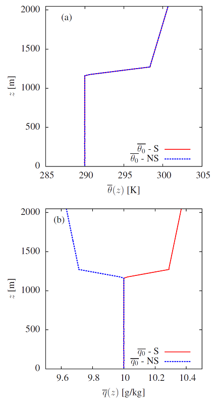 | Figure 1. Temperature (a) and specific humidity (b) for cases S and NS (S: specific humidity increases with z above the ABL; NS: specific humidity decreases with z above the ABL) |
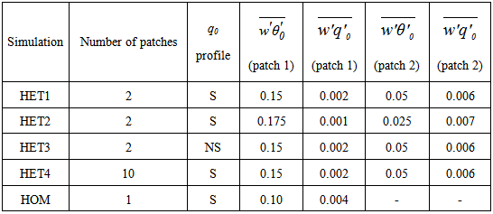
To introduce surface heterogeneity, the x-direction was divided into patches, and to each patch different surface fluxes were attributed. Five simulations were performed: in four of them, the x-direction was divided into two patches, one into ten patches and another one with only one patch to simulate a homogeneous surface. To maintain the control of the energy balance, the sum of sensible heat (H) and latent heat (LE) along the x-direction was set to be constant, namely | (1) |
where, | (2) |
and  | (3) |
ρ is the air density, cp is the specific heat and L is the latent heat of vaporization,  is the covariance between fluctuations of the vertical velocity component (w) and the potential temperature (θ), and
  is the covariance between the fluctuations of the vertical velocity component and the specific humidity q. Both fluxes were imposed as boundary conditions at z = 0 m. Values of surface fluxes and the number of patches in each simulation are presented in Table 1. Patch 1 has increased sensible heat flux and reduced latent heat flux compared to patch 2. Thus, the heterogeneity introduced by patches 1/2 can be interpreted as land/water or bare soil/vegetated patches on the land surface. In simulation HET4, with 10 patches, the fluxes of patch 1 were repeated for all odd patches, and the fluxes of patch 2 were repeated for all even patches. Note that for the simulations with 2 patches, patch length is larger than the ABL depth, while the case with 10 patches has a patch length smaller than the ABL depth. We anticipate that simulation HOM will produce perfect correlation. The decorrelation in simulations HET1, HET2, and HET4 are produced by the surface heterogeneity, while in simulation HET3 the entrainment fluxes also contribute to the decorrelation between temperature and specific humidity (see [9]).
Table 1. Number of patches, type of q0 profile (S: specific humidity increases with z above the ABL; NS: specific humidity decreases with z above the ABL), surface fluxes of temperature
 and specific humidity and specific humidity
 imposed as boundary conditions for patches 1 and 2 imposed as boundary conditions for patches 1 and 2
 |
| |
|
The LES setup described above produces temperature and specific humidity fields that are not statistically stationary, because their mean values increase with time. To circumvent this issue, instantaneous values of the scalar and velocity fields were stored every 5 seconds (frequency of 0.2 Hz) in 64×16×42 selected points. This resulted in a total of 43008 time series, analogous to a field experiment with measurements performed at 43008 points (or virtual towers) equally spaced (spatial resolution equal to 80×320×32 m3). Nonstationarity of the temperature and specific humidity was removed by applying a linear detrending to each time series, resulting in series that were approximately stationary (the same approach was used in [9], were more details can be found).
4. Results
In Figure 2, we present the x-z variation of the correlation coefficient, rθq, for simulations HET1 and HET2. The first detail to notice is that the strong heterogeneity case (HET2) has smaller correlation coefficients than the weaker one (HET1), as expected. In addition, the strong heterogeneity of HET2 produces decorrelations farther away from the ground. Above 400 m height, the scalar fields are typical of the mixed layer and there is virtually no influence of surface heterogeneity in the behaviour of rθq. An interesting feature that can be clearly observed in the simulation HET2 is that the correlation coefficient is smaller over patch 1 than over patch 2. This result is opposite to the one presented in [7], and probably reflects a difference between specifying surface fluxes (as done here) and surface values (as done in [7]).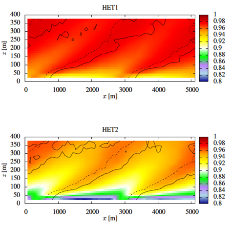 | Figure 2. x-z variation of the correlation coefficient rθq for simulations HET1 and HET2. Dashed lines show the IBL for mean temperature and solid lines show IBL for mean specific humidity |
Next we identify the internal boundary layers (IBL) for temperature and specific humidity. Figures 3 and 4 present the differences between the vertical gradients temperature and specific humidity and their horizontal averages over the entire domain. Following [10], we use the location where this difference is zero to identify the internal boundary layer (black lines in both figures). Thus, the IBL is given by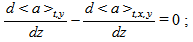 | (4) |
<a> is the average of a variable a − q or θ in this work. The regions within the IBL can essentially be viewed as the regions that are mostly influenced by a given patch.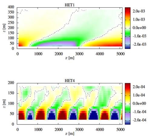 | Figure 3. Differences between vertical gradients of temperature (θ) in the first 400 m (HET1) and 200 m (HET4) from the vertical domain (obtained according to Eqn. 4). The time averages were obtained for the last hour of simulation, and black lines represent the internal boundary layer – simulations HET1 and HET4. Mean gradients are normalized using zi=2048 m and θ* =0.1840 K |
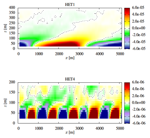 | Figure 4. Differences between vertical gradients of specific humidity (q) in the first 400 m (HET1) and 200 m (HET4) from the vertical domain (obtained according to Eqn. 4). The time averages were obtained for the last hour of simulation, and black lines represent the internal boundary layer – simulations HET1 and HET4. Mean gradients are normalized using zi=2048 m and q*=0.0075 gkg-1 |
We also investigate whether there is a height above which the heterogeneity effects are no longer present in the correlation coefficient. This can be done by applying the definition of blending height [10] to rθq. For our simulation setup, the blending height can be obtained from the deviations between the average of a in time and in the y-direction and the average in time and x,y−directions, this is, 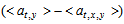 ; again, the blending height is located where this difference is zero. Here we use the method proposed by [10], in which a “neck” between the smallest and the largest quartile indicate the blending height. Results for simulations HET1, HET2 and HET4 are plotted in Figure 5.
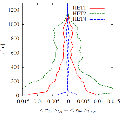 | Figure 5. Blending height estimative for simulations HET1, HET2 and HET4 |
We can observe in Figure 5 a clear “neck” for HET4 somewhere between 190 m and 210 m. However, it is difficult to identify a “neck” for simulations HET1 and HET2, suggesting that for patches larger than the ABL height, the surface heterogeneity may never be completely blended (at least for the correlation coefficient, given that Figures 3 and 4 suggest that mean temperature and specific humidity are fairly well blended). Figure 6−a presents the mean vertical profiles of rθq for all simulations. In the surface layer, the lowest correlation coefficient is observed for HET2, the simulation with the greatest difference between fluxes of the patches 1 and 2 (i.e. the strongest heterogeneity). For case HET3, rθq goes from ~0.9 to –1.0 because the entrainment fluxes of heat and water vapour have opposite signs due to the initial profile of specific humidity [9]. Note that for heights as low as ~100 m above the ground, the effects of entrainment are more pronounced than those caused by surface heterogeneity. This may not be the case for simulations with stronger contrast between the different patches, but it certainly emphasizes the strong effects of entrainment already noted by [9]. For simulations HET1, HET2 and HET4, the correlation coefficient rθq is presented as a function of x for z=56 m in Figure 6−b. It is interesting to note that the largest coefficients are observed approximately at the locations where the IBL lines for temperature are found (see IBL lines overlayed in Figure 2−b). 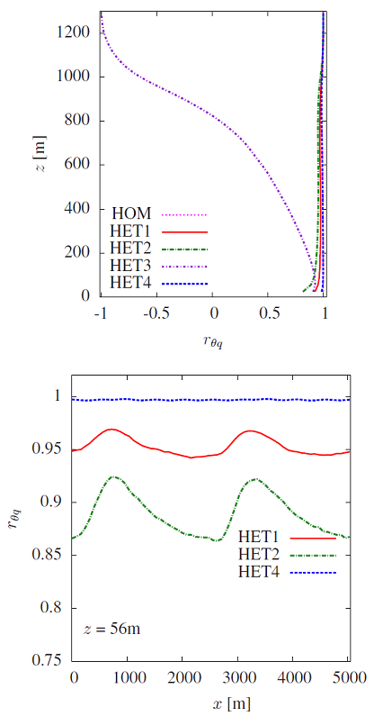 | Figure 6. (a) Vertical mean profiles of rθq for all simulations. (b) Horizontal mean profiles of rθq in x-direction for z=56 m for simulations HET1, HET2 and HET4 |
Figure 7 shows streamwise variation of q (Figure 7−a) and θ (Figure 7−b) variances, and  covariance (Figure 7−c) at z=56 m for simulations HET1, HET2 and HET4 – dimensionless values were obtained dividing the dimension values by turbulent scales θ* and q* ([9]). This figure suggests that most of the variation in the correlation coefficient can be explained by the variations in the variances themselves. These can be easily understood. As an example, the variance of the temperature is largest over the warmer patch and smaller over the colder one (so that in equilibrium σθ/θ* is the same over both surface). Thus, the streamwise variation of σθ can be understood through its production and dissipation terms. Note that there is an asymmetry between the increase and decrease in the variances shown in Figure 7−a,b, and these are related to the patterns of the correlation coefficient shown in Figure 6.
 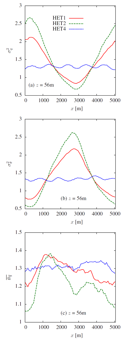 | Figure 7. Horizontal dimensionless mean profiles of q (a) and θ (b) variances, and  covariance in x-direction for z=56 m for simulations HET1, HET2 and HET4 covariance in x-direction for z=56 m for simulations HET1, HET2 and HET4 |
5. Discussion and Conclusions
The LES study presented here confirms that surface heterogeneity reduces the correlation coefficient between scalar fields. It also shows that: (i) stronger heterogeneity has a larger impact on the correlation coefficient between temperature and specific humidity; (ii) the main effect of surface heterogeneity on scalar dissimilarity influence occurs in the lower part of the atmospheric surface layer; (iii) effects of surface heterogeneity above the surface layer are very weak. Although rθq decreases with the increase of the difference between the fluxes of two contiguous patches, the reduction is not enough to decorrelate the scalars completely. The simulations also show a very large contrast between small patches and large patches (i.e. smaller/larger than the boundary layer height). While the former case has minimal effect on the correlation coefficient near the surface, the latter has a profound effect that remains very far downstream from the surface transition.It is also interesting to note that the lowest correlation coefficients were observed at the lowest grid point (located at a height of 24 m). In many field experiments, measurements are made at smaller heights. To get a better understanding about what happens below this height, it would be necessary to perform simulations with a greater vertical resolution (i.e., ∆z < 16 m).LES results could be used to plan field campaigns and interpret experimental results. To illustrate this possibility, suppose a hypothetical scenario in Figure 7, where the rθq for simulation HET2 is presented: suppose that the first half of the domain is covered by soil, and the second half is covered by water; in the field, an experimental station will be installed over the water in a distance of 2500 m from the soil-water border, and the measures will be performed at 4 m−height above the surface water. Most micrometeorologists would assume that the 2500 m fetch would be more than enough for the turbulence fields to equilibrate with the water surface. However, the simulations suggest that a significant reduction in the correlation coefficient due to the upwind transition may still be observed.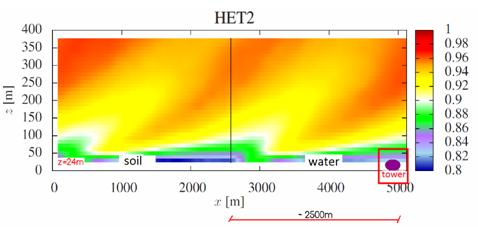 | Figure 8. (x,z) profile for rθq (simulation HET2) – hypothetical scenario to exemplify the use of LES results and field experiments |
These results can help interpret field experimental data such as the case discussed in [1]. Measurements were performed over a lake on a tower installed around 1400 m downwind from the margin and most of the time the correlation coefficients were significantly lower than 1 (62% of the time below 0.9 and 33% of the time below 0.8). LES results presented in [9] suggest that entrainment fluxes at the top of the ABL could explain the lack of similarity observed by [1]. Results presented here suggest that soil-water transition far upwind could also be the culprit.
ACKNOWLEDGEMENTS
This research was performed while Diana Maria Cancelli was a visiting student at the Department of Meteorology at The Pennsylvania State University with support from the Brazilian Science Without Borders program through CNPq/MCT (Process 201974/2011-8).
References
| [1] | Cancelli, D. M., Dias, N. L., and Chamecki, M. Dimensionless criteria for the production-dissipation equilibrium of scalar fluctuations and their implications for scalar similarity. Water Resour. Res., 48:W10522, 2012. |
| [2] | Andreas, E. L, R. J. Hill, J. R. Gosz, D. I. Moore, W. D. Otto, and A. D. Sarma (1998). Stability dependence of the eddy accumulation coefficients for momentum and scalars. Bound. Layer Meteor., 86, 409–420. |
| [3] | Asanuma, J.; Brutsaert, W. Turbulence variance characteristics of temperature and humidity in the unstable atmospheric surface layer above a variable pine forest. Water Resour. Res., v. 35, n. 2, p. 515-521, 1999. |
| [4] | Lamaud, E.; Irvine, M. Temperature-humidity dissimilarity and heat-to-water-vapour transport efficiency above and within a pine forest canopy: the role of the Bowen Ratio. Bound. Layer Meteorol., v. 120, p. 87-109, 2006. |
| [5] | Kumar, V.; Kleissl, J.; Meneveau, C.; Parlange, M. B. Large-eddy simulation of a diurnal cycle of the atmospheric boundary layer: Atmospheric stability and scaling issues. Water Resour. Res., v. 42, p. W06D09, 2006. |
| [6] | Albertson, J. D. Large Eddy simulation of land-atmosphere interaction. PhD Dissertation, Univ. of Calif., Davis, 185 pp. 1996. |
| [7] | Albertson, J. D. and Parlange, M. B. Natural integration of scalar fluxes from complex terrain. Advances in Water Resources, 23:239–252, 1999a. |
| [8] | Albertson, J. D. and Parlange, M. B. Surface length scales and shear stress: implications for land-atmosphere interaction over complex terrain. Water Resources Research, 35(7):2121–2132, 1999b. |
| [9] | Cancelli, D.M., Chamecki, M., Dias, N.L. A Large-Eddy Simulation Study of Scalar Dissimilarity in the Convective Atmospheric Boundary Layer. Journal of the Atmospheric Sciences, 71(1)3-15, 2014. |
| [10] | Bou-Zeid, E., Meneveau, C., and Parlange, M. B. Large-eddy simulation of neutral atmospheric boundary layer flow over heterogeneous surfaces: blending height and effective surface roughness. Water Resources Research, 40:W02505, 2004. |
 Abstract
 Reference
 Full-Text PDF
 Full-text HTML