1. Introduction

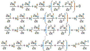
In present available literature increasing attention is paid to the task of searching for analytical solutions for the deterministic model governed by the advection-diffusion equation that allows to simulate contaminant dispersion in the planetary boundary layer. In fact, there exists an extensive literature to solve this kind of problem but for linearized versions, making the assuming the knowledge of the mean wind field. A variety of methods including the ones generating analytical representations for the solution are found. Among them, we mention the spectral GILTT technique (Generalized Integral Laplace Transform Technique), because this method solved a broad class of advection-diffusion problems for pollutant dispersion simulation in the atmosphere, considering appropriate eddy diffusivity for all atmospheric stability conditions as well as known wind profiles.

To this point it is important to emphasize that the GILTT (Generalized Integral Laplace Transform Technique) technique is a solution for the pollutant concentration that this expansion in the advection-diffusion equation and taking moments, we come out with a set of linear differential ordinary equations that may be solved analytically by Laplace transform technique [1-7]. A complete review of the GILTT method is given in [9] and references therein. The GILTT method was also applied to simulate radioactive pollution in atmosphere in accident scenarios [9] [10]. Recently some of the authors developed the 3D-GILTT method to solve the three dimensional advection-diffusion [11-15]. To reach that goal the spectral method was applied in the crosswind direction of the problem and the two dimensional resulting problem was solved by the GILTT method, where details may be found in [12]. Note that in all the works cited above the wind velocity field was known thus linearizing each of the studied problems.

The present work may be considered an extension of previous works, where the Navier-Stokes equation is coupled to the advection-diffusion equation. This extended model determines, besides the pollutant concentration also the mean wind field, which we assume to be the carrier of the pollutant substance. The coupled time dependent and two-dimensional advection-diffusion and Navier-Stokes equations are solved, following the idea of the decomposition method discussed by Adomian [16-18]. The basic idea relies on writing the coupled advection-diffusion and Navier-Stokes equation in a set of equations, in which the advective terms are linearized and the non-linear remaining advective terms are considered as source term. This equation system is then solved in a recursive fashion. In each set of coupled linear equations of the recursive system the source term is evaluated using the solution of the previous equation. Further, the first equation system, i.e. the recursion initialization is subject to the boundary conditions of the original problem, whereas the remaining equations of all subsequent recursions satisfy homogeneous boundary conditions.

To this end this article is organized as follows. In section 2 we present the mathematical model, the variable transformations, an order of magnitude analysis and some comments on the boundary condition dilemma. Section 3 presents the experimental dataset, the turbulent parameterization and the numerical results. We end, in section 4, with our conclusions and future perspectives.

2. Coupled Advection-Diffusion Navier-Stokes

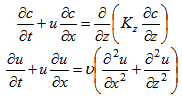
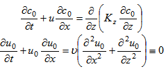
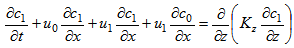
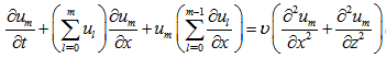
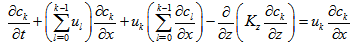
Our starting point is the 2 plus 1 dimensional space-time equation system composed by the advection-diffusion equation together with a reduced version of the incompressible Navier-Stokes equation:

(1)

Here t > 0, 0 < z < h and 0 < x < L, where h is the boundary layer height, L is the longitudinal extension of the domain, c denotes the mean concentration of a passive contaminant, u is the mean wind longitudinal velocity, υ is the kinetic viscosity and K_z is the vertical eddy diffusivity. The source condition is described by a short time emission point source that is implemented by the initial condition using the Dirac delta functional, which mimics a locally concentrated pollution substance at t=0. The boundary conditions are considered with zero flux at ground level and the top of the boundary layer respectively.

Note, that because of the term, velocity times velocity change along the wind propagation direction the problem is nonlinear, so that one has to resort to a method that allows to construct a solution in analytical representation without linear approximations. To this end, the pollutant concentration and the wind speed are expanded in a series and replaced in the equation system

(2)

Here, the expansion in c is used to apply the GILTT formalism documented in references [19] [20]. Due to the nonlinear character of the Navier-Stokes equation a separate formalism is proposed.

From the resulting equation a recursive set of linear coupled advection-diffusion and Navier-Stokes equation is constructed with the non-linearity considered as source term. Note, that the source term of the recursion initialization is identical zero by construction. Moreover, the construction of the recursion steps is not unique, and our specific choice allows to define the constitutive equations for all c_k and u_k such that the differential equation system is linear with the nonlinearities as source term. More specifically, the nonlinearity is decomposed in a way that the source term contains contributions from all previous recursion steps and thus is known. From the found solution, however with truncated series for c and u, numerical simulations are presented.

To the best of our knowledge this approach is novel since the equation for the wind field is coupled to the equation that models pollution dispersion and thus renders the problem self-contained. Previous approaches started from a known wind field, so that this sort of solution is not found in the literature.

The recursion initialization results in a problem already solved in previous works, whose the velocity term u₀ is constant and the advection-diffusion equation is solved for fixed velocity as for instance discussed in Moreira et al. (2009a),

(3)

Due of the peculiarities of the adopted initialization is subject to the initial and boundary conditions. All subsequent recursion steps have null initial and homogeneous boundary conditions.

(4)

In order to solve problem (4), taking advantage of the well-known solution of the stationary problem with advection in the x direction by the GILTT [20], we apply the Laplace Transform technique in the t variable. This procedure leads to a pseudo stationary problem:

(5)

where denotes the Laplace Transform of the concentration in the t variable .

Following the works [1, 2, 9] we pose that the solution of problem (5) has the form:

(6)

where are the eigenfunctions of the associated Sturm-Liouville problem, we mean, where are the respective eigenvalues.

To determine the unknown coefficient we replace Eq. (6) in Eq. (5) and taking moments, we mean applying the operator , we come out with the result:

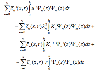(7)

Recasting Eq. (7) as a matrix ordinary differential equation, we read,

where is the column vector whose components are and the matrix F is defined like . The entries of matrices B₁, and B₂ are respectively given by:

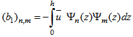and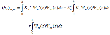

The integrals appearing in B₁ and B₂ are solved numerically via Gauss Legendre Quadrature.

Similar procedure leads to the boundary condition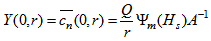, where A^-1 is the inverse of matrix A having the entry: .

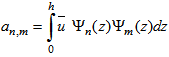Now, we are in position to solve problem (8), following the work [9], by the combined Laplace transform technique and diagonalization of the matrix H (H = XDX^-1). By this procedure we come out with the result

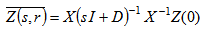(9)

where denotes the Laplace Transform of the vector Z(x,r). Here X is the matrix of the eigenvectors of the matrix H and X^-1 it is the inverse. The matrix D is the diagonal matrix of the eigenvalues of the matrix H and the entry of the matrix (sI + D) has the form {s + d_n}. Performing the Laplace transform inversion of Eq. (9), we come out:

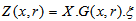(10)

where G(x,r) is the diagonal matrix with components . Further the new unknown arbitrary constant vector ξ is given by ξ = X^-1Z(0).

Once these unknown coefficients are evaluated we can construct the analytical solution to problem (6) applying the inverse Laplace transform definition. This procedure yields to the analytical result:

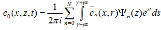(11)

By analytical, we mean that no approximation is made along the derivation of solution (11). To overcome the drawback of evaluating the line integral appearing in Eq. (11), in the sequel, we report a closed-form solution for this integral, using the Gaussian quadrature scheme. By this procedure we get:

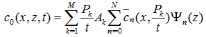(12)

where and are the weights and roots of the Gaussian quadrature scheme tabulated in the book of Stroud and Secrest [21]. Regarding the issue of the adopted Laplace numerical inversion scheme, it is important to mention that this approach is exact if the integrand is a polynomial of degree 2M-1 in the variable.

Before calculating the next correction term c₁ to the solution, we update de velocity field by u_1,

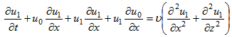(13)

By virtue this is a nonlinear equation and may be solved by the decomposition method as follows,

(14)

It is noteworthy that the recursive scheme (14) is organized in a way that the nonlinear terms left over from the previous decomposed equation is plugged into the subsequent equation as a source term. Once u₁ is determined the next term of the concentration explained may be evaluated

(15)

The general scheme that emerges consists of the nonlinear Navier-Stokes type equation that is solved following the analogue continuation of the recursion system (5)

(16)

Upon inserting the found term u_i into the advection-diffusion equation results in an equation that is solved using ortogonality in the spatial degrees of freedom and reducing the time dependence to a pseudo-stationary problem by Laplace transform,

(17)

3. Validation against Experimental Data

The solution procedure discussed in the previous section was coded in a computer program and will be available in future as a program library add-on. In order to illustrate the suitability of the discussed formulation to simulate contaminant dispersion in the atmospheric boundary layer, we evaluate the performance of the new solution against experimental ground-level concentrations.

3.1. Turbulent Parameterization

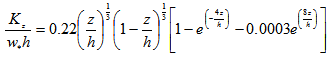
In atmospheric diffusion problems, the choice of the turbulence parameterization is a fundamental decision to model the pollutant dispersion. From the physical point of view the turbulence parameterization is an approximation to nature in the sense that we use a mathematical model as an approximated (or phenomenological) relation that can be used as a surrogate for the natural true unknown term, which might enter into the equation as a nonlinear contribution. The reliability of each model strongly depends on the way turbulent parameters are calculated and related to the current understanding of the ABL [22].

The present parameterization is based on the Taylor statistical diffusion theory and a kinetic energy spectral model. This methodology, derived for convective and moderately unstable conditions, provides eddy diffusivities described in terms of the characteristic velocity and length scales of energy-containing eddies. The time dependent eddy diffusivity has been derived by [23] and can be expressed as the following formula.

(18)

where h is the height (m) of the convective boundary layer, w_* is the vertical convective velocity (m/s).

3.2. Numerical Results

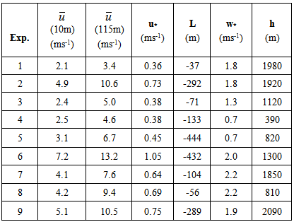
The measurements of the contaminant dispersion in the atmospheric boundary layer consist typically from a sequence of samples over a time period. The experiment used to validate the previously introduced solution was carried out in the northern part of Copenhagen and is described in detail by [24] [25]. Several runs of the experiment with changing meteorological conditions were considered as reference in order to simulate time dependent contaminant dispersion in the boundary layer and to evaluate the performance of the discussed solutions against the experimental centerline concentrations.

The essential data of the experiment are reported in the following. This experiment consisted of a tracer released without buoyancy from a tower at a height of 115m, and a collection of tracer sampling units were located at the ground-level positions up to the maximum of three crosswind arcs. The sampling unit distances varied between two to six kilometers from the point of release. The site was mainly residential with a roughness length of the 0.6m. The SF6 liberation started one hour before the sampling. The average of sample was of 1 h with 10 % of imprecisions. Table 1 summarizes the meteorological conditions of the Copenhagen experiment where is the mean wind velocity (m/s), L is the Obukhov length (m), h is the height of the convective boundary layer (m), w_* is the convective velocity scale (m/s) and u_* is the friction velocity (m/s).

Table 1. Meteorological conditions of the Copenhagen experiment [24]

The wind speed profile used in the simulations is described by a power law expressed following the findings of reference [26].

(19)

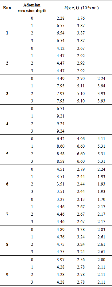
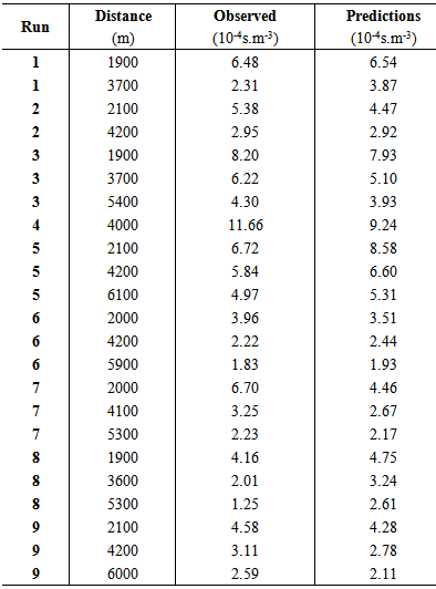
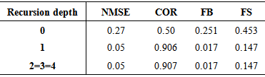
Here and are the horizontal mean wind speed at heights z and z₁ and n is an exponent that is related to the intensity of turbulence [27]. As is possible to see in [27], n = 0.1 is valid for a power low wind profile in unstable condition. Moreover, US EPA suggests for rural terrain (as default values used in regulatory models) to use n = 0.15 for neutral condition (class D) and n = 0.1 for stability class C (moderately unstable condition).

In order to exclude differences due to numerical uncertainties we define the numerical accuracy 10^-4 of our simulations determining the suitable number of terms of the solution series. As an eye-guide we report in table 2 on the numerical convergence of the results, considering successively one, two, three and four terms in the solution series. One observes that the desired accuracy, for the solved problem solved is attained including only four terms in the truncated series, which is valid for all distances considered. Once the number of terms in the series solution is determined numerical comparisons of the 3D-GILTT results against experimental data may be performed and are presented in table 3.

Table 2. Pollutant concentrations for nine runs at various positions of the Copenhagen experiment and model prediction by the new approach

Table 3. Pollutant concentrations for nine runs at various positions of the Copenhagen experiment and model prediction. The concentration is divided by the emission rate Q

To perform statistical comparisons between GILTT results against Copenhagen experimental data we consider the set of statistical indices described by [28] and defined by

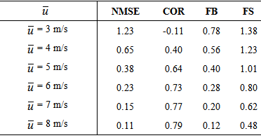
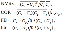where the subscripts o and p refer to observed and predicted quantities, respectively, and the bar indicates an averaged value. The best results are expected to have values near zero for the indices NMSE, FB and FS, and near 1 in the indice COR. Table 4 shows the findings of the statistical indices that show a fairly good agreement between the model predictions and the experimental data.

Table 4. Statistical comparison between the model results and the Copenhagen dataset, changing the mean wind (fixed value)

In Figure 1 the scatter diagram of model results against experimental data is presented. It can be realized that the present models in good agreement with the observations.

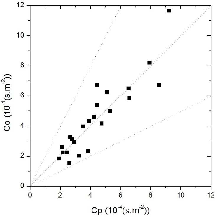Figure 1. Observed (Co) and predicted (Cp) scatter plot of centerline concentration using the Copenhagen dataset. Data between dotted lines correspond to ratio Co/Cp∈[0.5,2]

Table 5. Statistical comparison between the model results and the Copenhagen dataset

4. Conclusions

The present discussion considers a combined advection diffusion equation for pollution dispersion in the atmosphere together with the Navier-Stokes equation that describes the turbulent wind velocity field. To the best of our knowledge, until now there is no approach in the literature that treats pollution dispersion together with a dynamical equation for the wind field and with solution in analytical representation. In the literature there may be found a variety of Eulerian approaches [29-35] but none with a Navier-Stokes complement, so that in this sense the present formalism is new. Moreover, the fact that we derived the solution in a closed recursive fashion, allows to estimate, and thus control, the numerical error. To be more specific, after each recursion step the precision of the solution may be evaluated and the recursion depth is related to the prescribed accuracy. The recursive system is set-up circumventing linearization, so that in the limit of an infinite recursion depth the solution is manifest exact. This is attained organizing the non-linearity as a known source term using the solutions of the previous recursion steps. It is noteworthy, that the present version of the decomposition method, although inspired by Adomian's original work, is of pure differential form instead of using source terms with integrals.

Due to the construction of the model, the solution is adequate for moderate to strong wind velocities. The coupled advection-diffusion and Navier-Stokes equation describe only the mean values of concentration and wind velocity and thus have predominantly mechanical characteristics, although some thermal properties are already included in the eddy diffusivity parameterization. The authors are aware of the fact, that a more complete approach shall include also a coupling to an additional heat flux equation. A supporting argument is also manifest in the generated results for wind speeds between 3 m/s to 8 m/s (see table 4). The higher the wind speed, the better the correlations and the smaller the error, which indicates that from approximately 6 m/s, the model can be considered adequate. The omission of K_x is also compatible with these restrictions. Also the comparison of predicted to observed concentrations corroborate with these findings.

The present time dependent approach was restricted to the wind and vertical direction, only, however an extension to three dimensions is straight forward, due to the fact, that the linear solution (recursion initialization) is known independent of the dimensionality, and the recursion scheme follows the prescription presented in equations (5)-(8). In a future work we extend the approach to the full three dimensional model and in a subsequent step add effects due to entropy production by adding a thermal equation besides the mechanical description by Navier-Stokes.

ACKNOWLEDGEMENTS

The authors wish to thank CNPq (Conselho Nacional de Desenvolvimento Científico e Tecnológico), FAPERGS (Fundação de Amparo à Pesquisa do Estado do Rio Grande do Sul) for the partial financial support to this work.