1. Introduction

The study of flows over surfaces with temperature variability, or simply over surfaces whose temperature differs from the ambient temperature, has served as a challenge for scientists for many years. In this work, a special case of this type of flow is studied: stratified flow over surfaces with spatially uniform temperatures.

In this type of flow, the fluid is heated or cooled from below, possibly forming a stratified boundary layer, whose characteristics depend on stability. This type of situation occurs, for example, near the Earth surface in the atmospheric boundary layer. In this case, surface heating from the incident solar energy occurs during the day while surface cooling happens at night due to the emission of infra-red radiation.

The study of this type of flow has proven over the years to be very complex, especially due to the coupling of mechanical, thermal and transport phenomena to which it is subjected. Furthermore, this task requires a simultaneous understanding of the exchange processes of momentum, heat and sometimes moisture.

Here, a stratified and turbulent flow, i.e. subjected to high Reynolds numbers, is discussed. Many efforts have been made to understand this phenomenon, some depicting the conditions of similarity to which it can be associated (Kitaigorodskii, 1988), others seeking numerical solutions for the system of equations (Deardorff, 1972). Because of the inherent complexity of the numerical treatment of the Navier-Stokes and energy equations, and of the limitations of similarity theory for a complete study of this type of flow, the experimental simulation of atmospheric boundary layers in wind tunnels have been used to aid the understanding of this phenomenon.

In micrometeorology, the characterization of the atmospheric flow in conditions of stable stratification can be appointed as the most important current scientific problem. This happens because, in the night period when the surface radiative cooling is responsible for the formation of a stable layer, the turbulent intensities are drastically reduced compared to their corresponding values observed in the daytime. Two distinct types of stable boundary layer are observed (Mahrt, 1999). The first, typically referred to as weakly stable layer, occurs when the destruction of turbulence by thermal stratification is small in relation to the production of turbulence associated with vertical wind shear. In this case, although its intensity is reduced, the turbulence is temporally and spatially continuous. In the vertical, continuous turbulence is able to keep the surface connected by turbulence to the top of the layer. As a consequence, the atmosphere above the stable boundary layer (SBL) stays connected to the surface. A second type of SBL occurs when the destruction of turbulence, associated with the thermal stratification, is comparable to the mechanical production. In this case, the SBL is classified as very stable, and turbulence can be almost completely suppressed locally. Thus, there is no connection between horizontally separated locations and the air at lower levels is no longer coupled to the higher levels of the atmosphere. This way, the layers above the SBL do not exert influence in the variables observed at the surface. The very stable boundary layer is, in particular, the greatest current challenge for atmospheric boundary layer researchers, which not yet well understand various aspects related to it. Among these are the controls on the coupling state; the forcing for intermittent turbulent events, and their characteristics; the role of non-turbulent flows and how the various phenomena that occur simultaneously in the period, interact spatially and temporally. The SBL has been widely studied in recent years. Field observations are still the main tool for this purpose (Poulos et al., 2002; Sun et al., 2002; Acevedo et al. 2003; Banta et al, 2007; Acevedo et al., 2014; and others), but modeling studies (Duynkerke, 1988; Beare et al., 2006; Cuxart et al., 2006; Costa et al, 2011; and others) are also performed. These, however, are typically restricted to conditions of weakly stable layer, because the numerical schemes still have difficulty in reinstate the turbulent mixture once it is fully suppressed. Observations in wind tunnels have been used to study the turbulent flow in conditions of stable thermal stratification (Lienhard et al., 1990;. Yoon et al, 1990; Ohya et al., 1997; Ohya, 2001; Ohya et al, 2008). In these studies, vertical profiles of turbulent statistical moments are presented and it is analysed how they are affected by the thermal stratification. The aim of the present paper is to describe an initiative to study turbulent flow on a stable surface in a wind tunnel. Focus is given to the effect of the thermal stratification on different statistical moments of the turbulent field.

2. Experimental Setup

Experiments were performed in a wind tunnel at Instituto de Aeronáutica e Espaço (IAE/DCTA), São José dos Campos, Brazil. The wind tunnel is of a recirculation type having a rectangular test section, 1200 mm long, 720 mm wide, 500 mm high. Designed to produce thermally stratified flows, the test section was equipped with a cooling system. Such an apparatus consisted of an aluminum plate inserted at the bottom surface of the wind tunnel test section. In order to create a thermally stratified layer, the plate was cooled down to 5 °C, while the air entering the tunnel was kept at approximately 20 °C.

The experimental arrangement for stable boundary layer simulation is shown in figure 1. The boundary layer was artificially tripped by a 40-mm high fence at the entrance to the test section. The flow condition upstream of the fence is uniform with less than 2 % turbulence intensity. A stably stratified flow is created by cooling the test-section floor at around 5 °C, as shown in Figure 1. Stratified turbulent boundary layers with free stream velocities U from 1 to 5 m.s^-¹, varying at 0.5 m.s^-¹ steps have been created, covering a range of stabilities from weakly stable to neutral.

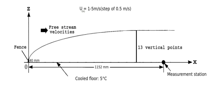Figure 1. Experimental Arrangement. (Adapted Ohya(2001))

The measurement of longitudinal wind speed was made at 1152 mm downstream from the fence. Tab. 1 shows the height from the tunnel surface, where the wind speed data were collected. The highest level was at the center of the tunnel. Data was acquired using a Dantec sensor system, 55P15-type (hot-wire) and an 56C01-type (cold-wire). The values of free stream velocities (U_∞), i.e., outside the boundary layer, were monitored with a pitot static tube in conjunction with a barometer Sensing Model GE Druck 610 DPI. The floor surface temperatures, was monitored with a digital multimeter FLUKE SERIE 170. For data acquisition, a sampling frequency of 1000 Hz was applied during a time interval of about 2 min.

Table 1. Vertical level distribution of measure points in the test section

3. Results and Discussion

3.1. Profiles Obtained from Hot-Wire Data

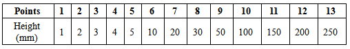
In this subsection, we present the profiles of quantities derived from observations made with hot wire anemometry. These are variables that depend only on the longitudinal wind fluctuations, in addition to observations of temperature.

The temperature profiles show the thermal stratification destruction provided by the turbulent mixing (Fig. 2). It is remarkable that the stability is much more intense in cases with low wind, decreasing progressively with increasing the mechanical forcing. Similar results have been obtained in simulations of wind tunnel (Ohya, 2001), but in that case the contrast was not so great because wind speeds were relatively more similar to each other than the values presented in Figure 2.

Figure 2. Mean temperature profiles as a function of wind speed as given by legend. In each case, the profiles were considered in relation to the temperature value at the highest level sampled

The greatest differences occur at lower levels, where the temperature is as much as 2.5 °C colder than at the top when the mean wind speed is 1.0 m.s^-1 (Fig. 3). In contrast, when the wind is 5.0 m.s^-1, the temperature of the lowest level is only 0.5 °C cooler than at the highest level, indicating an almost total destruction of the thermal stratification in this case.

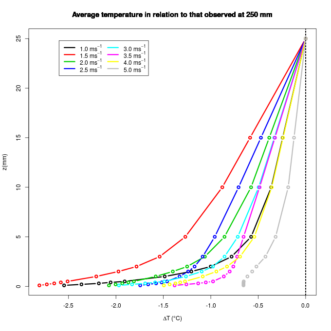
Figure 3. Temperature difference between the lowest and the highest level sampled a function of mean wind

The mean wind profile, in turn, is less affected by stratification that the mean temperature profile. This can be seen in Figure 4, which shows great similarity between the profiles of the stratified (upper left panel) and not stratified case (upper right). Anyway, the wind magnitudes in cases with stratification are always smaller than in the corresponding stratified cases. This is evidenced at the lower panel of Figure 4, which also shows that the wind reduction is proportionally larger in weak wind cases. Thus, for the experiment with 1 m.s^-1, the thermal stratification (more intense in this case) reduces the mean wind by 10%, while in cases with wind 4 or 5 m.s^-1, this reduction did not reach 5%. In all cases, the wind profile is approximately logarithmic up to a height of 100 mm, possibly associated with the barrier used at the entrance of the tunnel to maintain the turbulent layer.

With mean values of temperature and velocity, it is possible to determine the mean gradient Richardson number (Ri_g) for the layer. This is defined as

(1)

where g is the gravitational acceleration, θ is a reference temperature, Δθ is the potential temperature difference and ΔU is the the mean wind speed difference between two vertical levels separated by Δz.

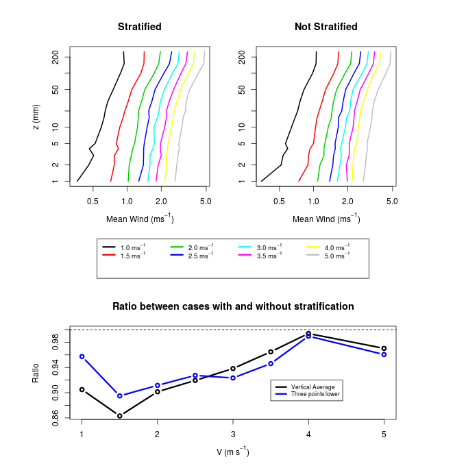Figure 4. Upper panels show the vertical profiles of mean wind speed for cases with (top left) and without stratification (top right). Lower panel shows the ratio between the value found with stratification to those without it, in average for the whole profile (black line) and for the three lowest points of observation (blue line)

The Richardson number compares an important mechanism for turbulence destruction in a stable environment, the thermal stratification, with the main production mechanism, which is associated with the wind shear. When destruction approaches production, the boundary layer is said to be very stable and turbulence may not be continuous.

In Table 2, the values of Ri_g for each experiment, calculated from differences between the highest and lowest observational levels are shown. The most stable cases are associated with larger Ri_g, but it is crucial to note that even the more stable cases are far from the limit of non-continuous turbulence, generally observed when R_g is above 0.2. This suggests that all experiments are representative of a weakly stable layer in which the turbulence is always continuous. Cases with stronger wind, where Ri_g is close to 0.01, are representative of an approximately neutral layer.

Table 2. Vertical temperature gradients and wind gradient and the Richardson number for each experiment performed hot wire

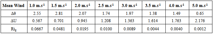
The greatest influence of the thermal stability is in the velocity fluctuations, as can be expected by the turbulent kinetic energy (TKE) budget equation, which determines that under stable conditions, there is turbulence destruction associated with the vertical temperature gradient.

Thus, it is expected that in low wind cases, when the vertical temperature gradient is greater (as shown in Fig. 2), there should be a notable reduction of turbulent fluctuations. This is, indeed, observed in Fig. 5. The variance of the turbulent fluctuations is approximately constant up to 100 mm, a layer that coincides with the logarithmic vertical profile of the mean wind. Ohya (2001) observed that in most cases of static stability the magnitude of the velocity fluctuations showed a peak near the surface. Such a peak was not observed in this study for any stability case. In contrast, in all cases, the turbulent velocity fluctuations were nearly constant in magnitude for an entire layer from the surface to 100 mm. The greatest reduction of velocity fluctuations from the case with no stratification to the stratified case occurred the case at the 1.5 m.s^-1 experiment when it reached 40% (Fig. 4, bottom panel). In general, cases with less wind (and consequently increased thermal stratification) had the largest reductions of the wind variance by the thermal stratification. When the wind reaches 4 to 5 m.s^-1, this reduction did not reach 10%.

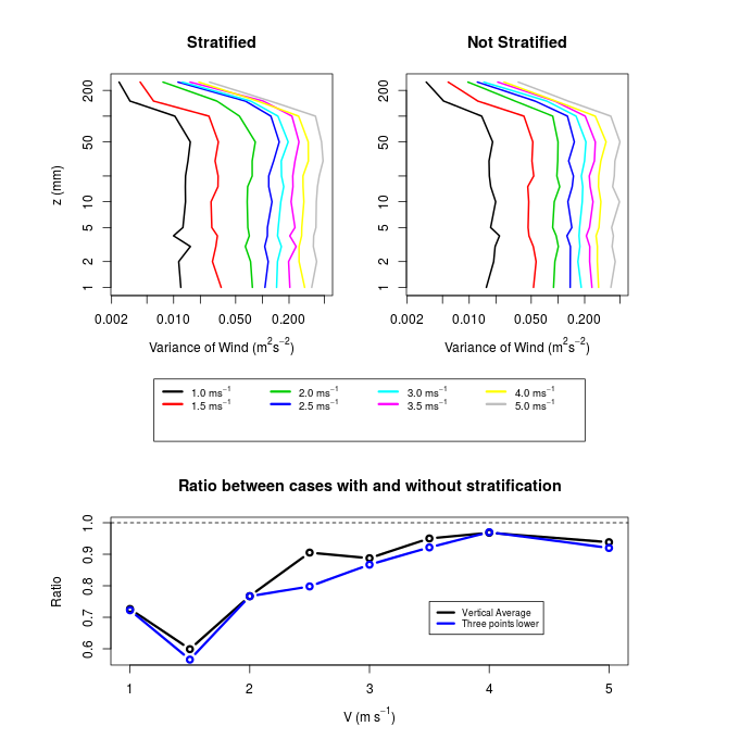Figure 5. Same as in figure 4, but for the variance of the longitudinal wind fluctuations

Vertical profiles of the third and fourth moments of the turbulent fluctuations have also been determined. The third central moment is associated with the skewness through expression

(2)

where are the turbulent fluctuations of longitudinal velocity, is the average operator and σ_u is the standard deviation of u. This coefficient indicates whether there is a more common direction of the velocity fluctuations around the average, being zero for a perfectly symmetrical distribution. Equivalently, the kurtosis is defined as

(3)

and quantifies the "flattening" of the distribution around the mean value, with the value 3 for a Gaussian distribution and greater than that for a more widespread distribution than normal. The profiles indicate positive skewness from the surface to approximately 50-mm height in both stratified and not stratifed cases (Fig. 6). Above 50 mm, there is a rapid decrease in the skewness coefficient, which reaches large negative values at 150 mm.

In this same region of the positive skewness, kurtosis approaches 3 in both cases, the same value as in a normal distribution (Fig. 7). At the heights where skewness is negative, kurtosis reaches a maximum. Interestingly, the negative peaks of skewness and positive kurtosis coincide with the region where the wind profile ceases to be logarithmic (Figure 4), and it is also where the variance of the wind decreases dramatically in relation to an approximately constant value at lower levels. Other studies in the wind tunnel (Choi and Clayton, 2001; Choi and Orchard, 2001) identified maximum skewness or kurtosis similar to those found here.

It is interesting to notice that the third and fourth order moments appear to be little affected by stratification, since in both cases (Figures 6 and 7, bottom panels) the ratios between the values observed in each case approach unity for all wind speeds considered.

Figure 6. Same as in figure 4, but for the skewness coefficient. In the upper panels, dotted line represents zero

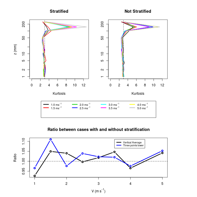Figure 7. Same as in figure 4, but for the kurtosis coefficient. In the upper panel, the dotted line indicates the value 3, typical of a Gaussian distribution

3.2. Profiles Obtained Data PIV

Vertical velocity fluctuations data are only available through particle images velocimetry (PIV). These are needed for determining some relevant quantities in a stable boundary layer, such as vertical turbulent fluxes and vertical eddy diffusion coefficients. It is important to note that, in general, the data presented here show more scatter than in the previous section, and this is mainly due to the different observation technique used.

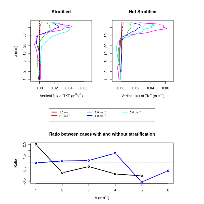
The vertical profiles of the turbulent flux show a maximum in both stratified and not stratified cases at heights between 50 and 100 mm for all wind speeds (Fig. 8). Similar profiles have been observed in previous studies that reported experiments of wind tunnel with flow over vegetated areas (Brunet; Finnigan; Raupach, 1994; Zhu et al., 2006; Zhu; Hout; Katz, 2007). In these studies, the peak of momentum flux coincides with the height of the roughness elements used. This suggests, therefore, that the maximum observed here is associated with the fence of 40 mm used to maintain a boundary layer with well-developed turbulence in the simulations. The momentum flux is affected by stratification, and this influence is greater in levels near the surface. This is shown in the bottom panel of Figure 8, which shows that the first 10 levels of PIV observation, when the wind is 1 m.s^-1, the magnitude of in the stratified case corresponds to only 40% of the value of no stratified case. In the vertical average, the reduction is smaller, but still substantial, where the value of the stratified case corresponding to 75% of that observed in the condition without stratification. The difference between the two cases is reduced with winds of 2 m.s^-1 and becomes almost non-existent for winds of 3 m.s^-1 or more intense.

It is also possible to determine from the data of PIV the turbulent vertical flux of turbulent kinetic energy (TKE) (Fig. 9), defined as half of the sum of the variances of the three wind components. In this case, it is important to emphasize that this is not the TKE itself, but the contributions of the variances of the u and w components, available in the measurements of PIV. Thus, the flux is the amount , where Of all the variables presented here, this presents the greatest statistical uncertainty, because it is a third moment obtained from the PIV data. Anyway, a significant pattern is noticeable, with negative fluxes in the lower levels and positive values aloft. The large fluctuations observed do not allow any conclusions with respect to differences between stratified and not stratified cases.

Finally, PIV data also allow to obtain the eddy diffusivity coefficients of momentum (Fig. 10). This is defined as the coefficient of proportionality between the turbulent fluxes of momentum and the vertical gradients of velocity, being therefore determined as

(4)

The K_m profiles increase from the surface, reaching a maximum near 50 mm. This peak is broad, and in some cases is not well defined, due to the need of smoothing the wind speed vertical gradients. However, regardless of the uncertainties, some significant patterns are evident. Diffusivities are significantly lower for cases with weak wind. Furthermore, the stratification reduces significantly the coefficients when the wind is 1 or 2 m.s^-1, which corresponds to the cases of more intense stratification. This reduction is higher near the surface, reaching in the 3 first levels of observation, a decrease of 60% with regard to the case lacking stratification when the wind is 1 m.s^-1. The same reduction reaches 30% when averaged for all vertical levels The main patterns shown in Figure 10 are in agreement with those presented by Ohya (2001), who observed, as well as in the present study, profiles of K_m increasing from the surface to find a broad maximum, and a strong influence of stability on the values coefficients. The shape of the profiles is also in agreement with those observed by Brunet et al. (1994), which did not analyze the dependence with stability.

The results obtained so far show that, even though the thermal stratification is not intense (as evidenced by the low values of Richardson number), there is a influence of thermal stratification over the flow, significantly reducing velocity fluctuations in the more stables cases. Unfortunately, the system used does not permit the determination of the thermal destruction term of turbulence in the turbulent kinetic energy equation. This term is given by:

(5)

where is the vertical turbulent sensible heat flux, and it is impossible to be determined due to the absence of measurements of the fluctuations of temperature and vertical velocity in the same system of measurement. On the other hand, it is possible to make a qualitative estimation of this term, estimated by the traditional theory K, which relates fluxes to the vertical gradients through the turbulent diffusivities by the expression

(6)

where is the turbulent diffusivity of sensible heat and is the vertical temperature gradient, shown in Figure 2. Ohya (2001) shows that for values Richardson number smaller 0.1 the relationship between turbulent diffusivity of sensible heat and momentum is approximately constant and equal to K_h/K_m = 0.8. Thus, one can use the eddy diffusivity coefficients of momentum shown in Figure 10, together with the vertical temperature profiles (Figure 2) for estimating the term thermal destruction of turbulence. It is also important to normalize the data to obtain an estimate of the importance of this term in relation to other terms of the balance equation of TKE.

To normalize the thermal destruction term was chosen the dissipation term, which is obtained from the structure function, and represents an independent measure of the PIV observations. The results are shown in Figure 11 and confirm the most important role of thermal destruction in the case of weak wind, when the thermal stratification is more intense. The destruction of turbulence by thermal stratification reaches a maximum between the height of 1 and 10 mm, where there is sufficient turbulent diffusivity, with a temperature gradient still appreciable. With wind 1 m.s^-1, the estimated thermal destruction reaches 0.8% of the average dissipation, while in high wind conditions this value does not reach 0.1%. Anyway, it is important to note that in all cases the thermal destruction estimated in this way is smaller than the dissipation rates, while the observed reduction of the variances of speed when the wind is weak indicates that the thermal destruction must have rather a relevant role. We attribute this discrepancy partially to the uncertainty associated with the use of different observational techniques, and therefore cannot show a reliable closing balance of TKE. Nevertheless, it is important to notice that atmospheric boundary layer studies in weakly stable conditions have shown the buoyant destruction to be at least one order of magnitude smaller than the dissipation rate (kosovic; Curry, 2000; Shah; Bou-Zeid, 2014).

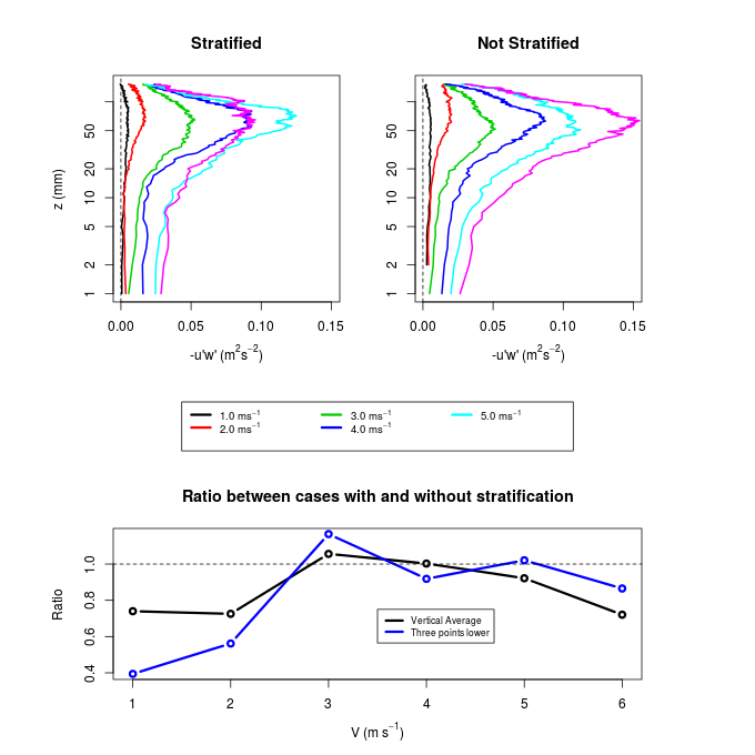Figure 8. Same as in figure 4, but for the absolute values of turbulent momentum fluxes

Figure 9. Same as in figure 4, but for turbulent vertical flux TKE

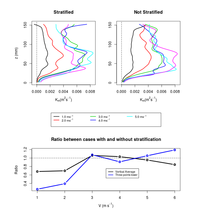Figure 10. Same as in figure 4, but for the eddy diffusivity coefficients of momentum

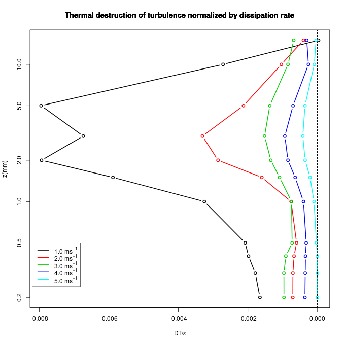Figure 11. Thermal destruction Term, estimated as described in the text for different values of wind velocity. In each case, the profiles were normalized by the vertical average rate dissipation

4. Conclusions

The experiments performed in a wind tunnel over a cooled surface presented in this paper allowed us to obtain some interesting results. Among these are:

- A stratified layer is formed, however, quickly destroyed by winds of moderate intensity. Even in the case of weak wind of 1 m.s^-1, the stratified layer that was formed could not be characterized as a very stable boundary layer having Richardson number below 0.1;

- Even not being a very stable stratification, other quantities associated with turbulent flow, in addition to the temperature profile showed substantial reduction in cases of weaker wind. Among these, we highlight the variances of the turbulent velocity fluctuations, the dissipation rate, the vertical turbulent fluxes of momentum and eddy diffusivity coefficients;

- Other quantities were not significantly affected by thermal stratification. Among these, the most relevant is the average wind profile. Statistical moments of third (skewness) and fourth order (kurtosis) also had no relevant changes between stratified and not stratified cases.

ACKNOWLEDGEMENTS

The authors are gratefully indebted to Capes (Coordenação de Aperfeiçoamento de Pessoal de Ensino Superior, Brasil), CNPq (Conselho Nacional de Desenvolvimento Cientíico e Tecnológico, Brasil) for the financial support of this work and DCTA (Departamento de Ciência e Tecnologia Aeroespacial) for the technical support.