A. C. Akpanta, I. E. Okorie
Department of Statistics, Abia State University, Uturu, Nigeria
Correspondence to: A. C. Akpanta, Department of Statistics, Abia State University, Uturu, Nigeria.
| Email: |  |
Copyright © 2014 Scientific & Academic Publishing. All Rights Reserved.
Abstract
This paper used Box-Jenkins Techniques in Modelling and Forecasting Nigeria Crude Oil Prices obtained from 1982 to 2013 from the Central Bank of Nigeria’s website. The descriptive statistics obtained showed, among other statistics, the mean to be 40.63USD/Barrel with a standard deviation of 32.28. The Augmented Dickey -Fuller test revealed that the time series data was unit root non-stationary. First order differencing was done to coerce the non-stationary time series into a stationary one - a condition that allowed the use of the univariate Box- Jenkins modelling approach. The time series, the ACF and the PACF plots of the first order difference of the crude oil price data suggested ARIMA(6,1,7). It was discovered that a lot of the model parameters was redundant hence settling for only statistically significant parameters of the model resulted to fitting ARIMA( 2,1,2) which led to a reduced and parsimonious model. From the diagnostic plots, an overall consistency with the white noise process was noticed. The paper further compared the two models on the basis of their information criterion statistics and ARIMA (2, 1,2) fared better and was used to make forecast. Comparison of the actual/observed prices from January to July 2014 was done with their corresponding forecast values and a t-test of significance showed no significant difference.
Keywords:
ARIMA, Crude oil prices, Forecast, Stationarity, Univariate time series data
Cite this paper: A. C. Akpanta, I. E. Okorie, Application of Box-Jenkins Techniques in Modelling and Forecasting Nigeria Crude Oil Prices, International Journal of Statistics and Applications, Vol. 4 No. 6, 2014, pp. 283-291. doi: 10.5923/j.statistics.20140406.05.
1. Introduction
In Nigeria, the petroleum industry is the largest industry and main generator of GDP with statistics that oil revenue has totalled $340 billion in exports since the 1970s. She has a maximum crude oil production capacity of 2.5 million barrels per day and ranks as Africa's largest producer of oil and the sixth largest oil producing country in the world [1]. Undoubtedly, many works have been done and are still being done globally on this major income-earning industry - the crude oil. For example, in modelling and forecasting crude oil prices, some scholars have used classical time series models like autoregressive moving average (ARMA) [2], others econometric model like generalized autoregressive conditional heteroscedasticity (GARCH) [3]. Others have also attempted the forecast using asymmetric cycles on crude oil prices [4]. Shabri and Samsudin [5] used a more complex approach in forecasting the price.In this paper titled ‘the application of Box-Jenkins techniques in modelling and forecasting Nigeria crude oil prices’, a near up-to-date analysis of the prices of crude oil in Nigeria (from January 1982 to December 2013 [6]) is attempted. This has not been done before now.The motivation is derived from the fact that reliable and adequate estimates of crude oil prices are very essential for planning and policy-making by not only the government but international agencies as well.
2. Methods
Since the data is indexed in time, time series analysis becomes an appropriate statistical technique to implore [7].
2.1. Time Series Analysis
Generally, a time series, as a stochastic process, is an ordered sequence of observations made sequentially in time. The most important feature of such data is the likely lack of independence between successive observations in time. Time series data can be univariate as is the case with the crude oil prices under consideration or multivariate.The ARIMA (Auto Regressive Integrated Moving Average) class of model is only applied to a univariate time series data. This method of time series modelling is often referred to as the Box-Jenkins approach. The act of ARIMA modelling gained its credence from Box and Jenkins 1976, [8]. A good ARIMA model requires at least 50 observations and a reasonably large sample size is required for a seasonal time series [9]. With the ARIMA models forecast are made using the past of the process and are particularly suitable for short term forecasting and also forecasting seasonally enriched series. Box-Jenkins models are only reasonable for stationary time series with equi-spaced discrete time intervals. A time series is said to be stationary if its mean, variance and autocorrelation functions remains unchanged over time. However, in practice many time series data are non-stationary and could be transformed to stationarity by a simple differencing exercise, usually the first difference is enough to coerce a non-stationary time series into a stationary one and the second difference is seldom required. Non-stationarity implies trend and is typically induced by serial correlation.
2.2. Definition
Let  denote a non-stationary time series which could adequately be modelled by the ARIMA (p,d,q) model defined by:
  | (1) |
where  denote the order of the AR part of the model,
  denote the order of the MA part of the model and
  denote the number of times the non-stationary time series need to be differenced to make it stationary. Interestingly, when
 , (1) reduces to a stationary ARMA (p,q) process defined by:
 | (2) |
where  and
and  are as defined above.
2.3. Non-Stationary Process
The random walk process: | (3) |
is an example of a non-stationary process. Where,  depends on the immediate past of the process and
  is essentially a stationary white noise process i.e.
  Applying the first differencing to (3) we have:
 | (4) |
hence,  is a white noise process and stationary.
2.4. Box-Jenkins Procedures
The objective of Box-Jenkins modelling approach is to find a parsimonious ARIMA model that describes the inherent generating process of the observed time series. The Box-Jenkins model building consists of three stages namely-identificatison, estimation and diagnostic checking stages.The identification stage involves selecting one or more ARIMA model(s) based on the estimated ACF and PACF plots. The ACF plot of the AR (Auto Regressive) process decays exponentially to zero and its PACF plot shows cut-off to zero after lag . The ACF plot of the MA process shows cut-off to zero after lag
  while its PACF decays exponentially to zero. The combination of the AR (P) and the MA (q) processes is known as the ARMA (p,q) process (Equation 2) which has ACF and PACF that decays exponentially to zero. The maximum likelihood estimation method could be used in the estimation stage to estimate the parameters of the identified model(s). The last stage (diagnostic checking) involves assessing the validity of the identified and fitted models through possible statistically significant test. Finally, the best fitting ARIMA model would be used to make forecast.
3. Results and Discussions
3.1. Data Analyses
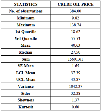
The data on the Crude Oil Prices (USD/Barrel) was analysed using R (statistical software), [10] and the following results obtained: Table 1. Descriptive Statistics for the Crude Oil Price Data
 |
| |
|
From Table 1 above it could be seen that the crude oil price did not fall below 9.82 USD/Barrel and did not rise more than 138.74 USD/Barrel from January 1982 to December 2013 with an average crude oil price of 40.63 USD/Barrel. Also, the crude oil Price data is positively skewed and heavy tailed, hence not normally distributed.Let  denote the time series of Nigeria crude oil price in USD (January 1982 - December 2013). We present the time series plot, ACF plot and the PACF plot of the crude oil price data as follows:From the time series plot (Top panel) of Nigeria crude oil price in USD/Barrel in Figure 1, it could be seen that the series shows an overall fluctuation. It also appears to be relatively stable from January 1982 to about the first Quarter of 2000 where a substantial upward trend followed immediately; and thereafter a sharp fall at about the last Quarter of 2008, followed by a price increase at about the first Quarter of 2009 which persisted until December 2013. The presence of trend in the series suggests a non constant mean over time. The ACF plot (Centre panel) decays very slowly to zero where these observations from the time series plot and the ACF plot imply a non-stationary time series. The PACF plot (Bottom panel) has a cut-off at lag 1 suggesting an AR(1)
  model for the crude oil price data. Although, the crude oil price data has through the above visual inspection shown non-stationarity, an AR (1) model is fitted to the data as suggested by the PACF.
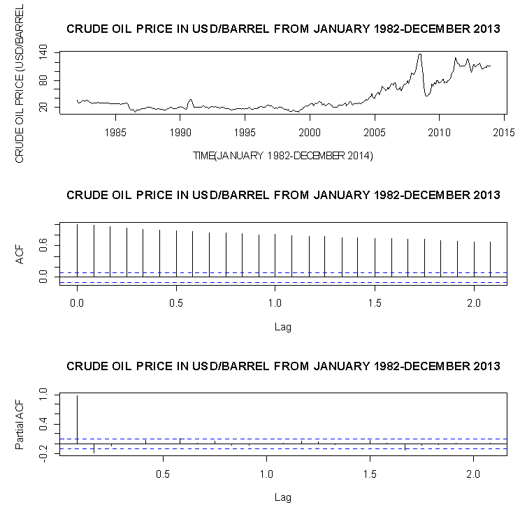 | Figure 1. Corresponds to the plot of the ordinary series of Nigeria Crude Oil price in USD/Barrel (Top-plot), the ACF plot of the ordinary series (Centred-plot), and the PACF plot of the ordinary series |
From the information in Table 2, we could see that the fitted AR(1) model parameter is statistically significant due to an associated very small standard error which is more than two times smaller than the estimated model parameter  Hence, the diagnostic plots in Figure 2.
Table 2. AR(1)
 model fitting model fitting
 |
| |
|
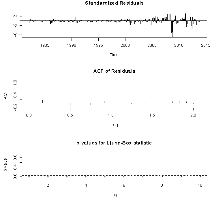 | Figure 2. Diagnostic plots for the fitted AR (1)  model on the basis of the standardized residuals model on the basis of the standardized residuals |
The diagnostic plots show that the fitted model is not good because its standardised residuals are not consistent with the white noise process. This is because the plot of the standardised residual has spikes concentrating more on the negative region of the graph particularly from 1982 to about 2000 and also an alternating batches of spikes could be seen in 2008 and 2009, these suggests that the standardised residuals are not normally distributed. The ACF plot shows a substantial spike at lag 1 and the p-values of the Ljung-Box statistic [11] fall below the 0.05 band (dashed lines) indicating very small p-values  where these observations imply that the standardised residuals are correlated hence, not normally distributed. Consequently, a test (the Augmented Dickey-Fuller test [12]) to further substantiate the suggestive non-stationarity that is based on the subjective visual display of the time series plot is carried out in section 3.2.
3.2. Test of Hypothesis on Stationarity of the Data
H0: The time series data is unit root non stationaryH1: The time series data is stationaryTable 3. The Augmented Dickey-Fuller Test
 |
| |
|
Decision: Large p-value greater than 0.05 is in favour of the null hypothesis. Thus, we accept the null hypothesis at 5% level of significance that the time series is unit root non stationary. In order to coerce the non stationary time series into a stationary one to enable the univariate Box-Jenkins modelling approach, we take the ordinary first difference denoted by:  or
or  Presented in Figure 3 are the time series plot, ACF plot and the PACF plot of the first ordinary difference of the crude oil price data.
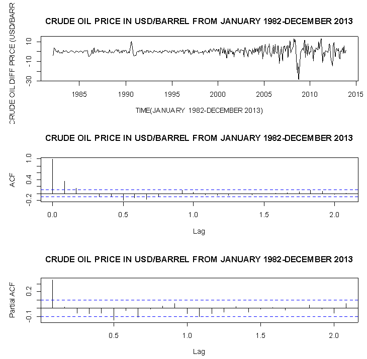 | Figure 3. Corresponds to the plot of the first differenced series of Nigeria Crude Oil price in USD/Barrel (Top-plot), the ACF plot of the first differenced series (Centred-plot), and the PACF plot of the first differenced series |
From the time series plot (Top panel) of Nigeria crude oil differenced prices in USD/Barrel in Figure 3, it could be seen that the series shows an upward and downward movement about zero hence, no trend pattern. The ACF plot (Centre panel) also shows a sinusoidal quick decay pattern which suggests stationarity and a cut-off at lag 7. The PACF plot (Bottom panel) has a cut-off at lag 6 these observations from the ACF and PACF plots suggests an


 or
or
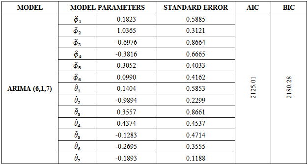
 model for the crude oil price data. From the information presented in Table 4, we could see that the following model parameters:
  of the fitted ARIMA (6,1,7) model are redundant (not statistically significant) due to their associated standard errors which are more than two times larger than the estimated model parameters. Hence the diagnostic plots are as follows:
Table 4. ARIMA(6,1,7)
 model fitting model fitting
 |
| |
|
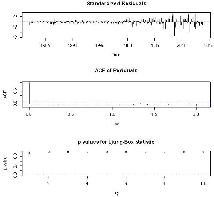 | Figure 4. The diagnostic plots for the fitted ARIMA(6,1,7)  |
The diagnostic plots of the fitted ARIMA (6,1,7) suggest an overall consistency of the standardised residuals with the white noise process which further implies a good fit of the fitted model to the crude oil price data. This is because the standardized residual plot shows no pattern and swings about a common value of zero, the ACF plot of the standardized residuals shows no spike across lags which implies that the standardized residuals are uncorrelated and the p- value plot of the Ljung-Box statistics shows that all the p-values of the autocorrelation functions, at various lags, are very large  . Clearly, in support of the ACF plot. However, the redundancy of a large number of the fitted model parameters would undermine the adequacy of the fitted ARIMA (6,1,7) model. But since
  and
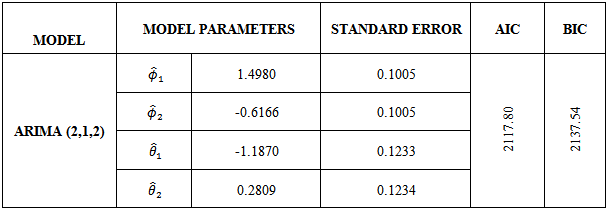
and  are the only statistically significant parameters of the model it therefore suggests that the ARIMA (2,1,2) be fitted to the crude oil price data leading to a reduced and parsimonious model.Clearly, from Table 5 all the model parameters are statistically significantly different from zero as suggested by the small standard errors corresponding to the ARIMA (2,1,2) parameters. The diagnostic plots are immediately presented in Figure 5.
Table 5. ARIMA(2,1,2)
 Model fitting Model fitting
 |
| |
|
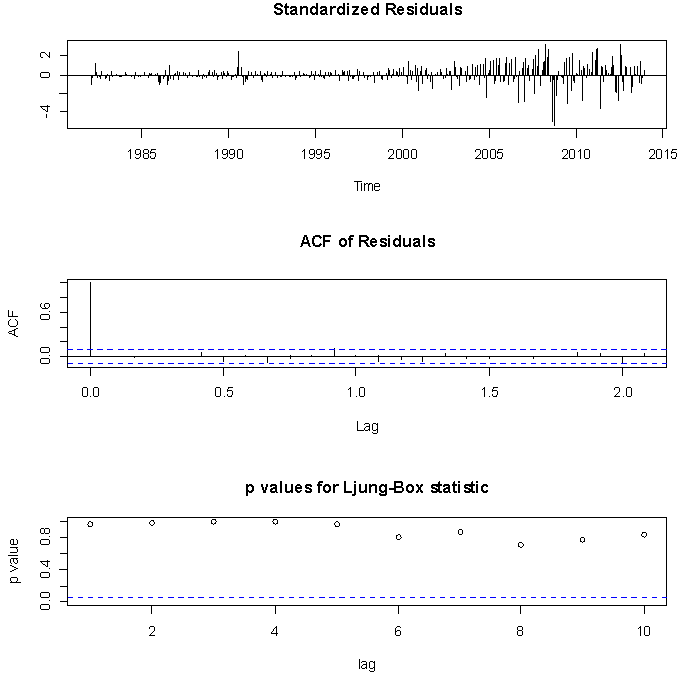 | Figure 5. The diagnostic plots for the fitted ARIMA (2,1,2)  |
Table 6. Model Selection
 |
| |
|
From the plots we could see that the standardised residuals are normally distributed because the spikes are evenly distributed about a common zero mean, the ACF plot shows at 5% level of significance that the standardised residuals are uncorrelated at various lags and all the p-values for the Ljung-Box statistics are very large, suggesting that the set of the autocorrelation coefficients at various lags of the standardised residuals are not significantly different from zero. Hence, depicts an overall consistency with the white noise process.We therefore compare the emergent two models on the basis of their information criterion statistics particularly, the Akaike information criterion (AIC) [13] and the Bayes information criterion (BIC) [14] where the model with the smallest information criterion statistics implies the model with the highest maximised log-likelihood hence, the best fitting model. Given the information in Table 6 above the ARIMA(2,1,2) model with the smallest AIC and BIC statistics has emerged as the best fitting model for the underlying generating process of the crude oil price data and would further be used to make forecast.The reliability and accuracy of the forecast crude oil prices would be ascertained by a mere comparison of the observed prices and the point forecast price values through the two sample t-test as presented below. Note that we have restricted the test to very few forecast values (January 2014 to July 2014) because long term forecast is not advisable for obvious reason.
3.3. Test of Hypothesis on Difference of Two Means of the Forecast and the Observed Values
H0: Difference in the mean of the observed crude oil prices and mean of the forecast crude oil prices ≠ 0H1: Difference in the mean of the observed crude oil prices and mean of the forecast crude oil prices ≠ 0From the information presented in Table 8 above we could reasonably conclude at 5% level of significance that the difference between the observed crude oil price values and the forecast price values are equal to zero or more technically not statistically significantly different from zero. This conclusion is made on the basis of the large p-value of 0.0939 which is greater than 0.05. Alternatively, it could equally be inferred from the 95% confidence interval (-0.2682, 2.9811) because the interval contains zero.
4. Conclusions
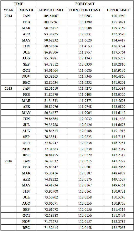
The work considered 372 months’ data on crude oil prices in Nigeria from January 1982 and from Table 1, the mean and the standard deviation were found to be 40.63USD/Barrel and 32.28 respectively. From the Augmented Dickey-Fuller test summarised in Table 3 the null hypothesis, at 5% level of significance, that the time series is unit root non stationary cannot be rejected. Hence, first order differencing was done to coerce the non-stationary time series into a stationary one - a condition that allowed the use of the univariate Box- Jenkins modelling approach. The time series, the ACF and the PACF plots of the first order difference of the crude oil price data suggested ARIMA(6,1,7). From the information presented in Table 4, most of the parameters of the fitted model are not statistically significant due to their associated standard errors which are more than two times larger than the estimated model parameters. Hence, only statistically significant parameters were upheld and that resulted in fitting ARIMA(2,1,2) which led to a reduced and parsimonious model. From the diagnostic plots, an overall consistency with the white noise process was noticed. Given the information in Table 6, the ARIMA(2,1,2) model with the smallest AIC and BIC statistics emerged as the best fitting model for the underlying generating process of the crude oil price data and was used to make forecast. Comparison of the actual/observed prices from January to July 2014 was done with their corresponding forecast values and from Table 8 we could reasonably conclude, at 5% level of significance, that the difference between the observed crude oil price values and the forecast price values are statistically not significant from zero.Table 7. The 95% Confidence Interval for the 3 Years Crude Oil Price Forecast (January 2014-December 2016)
 |
| |
|
Table 8. Two sample t-test
 |
| |
|
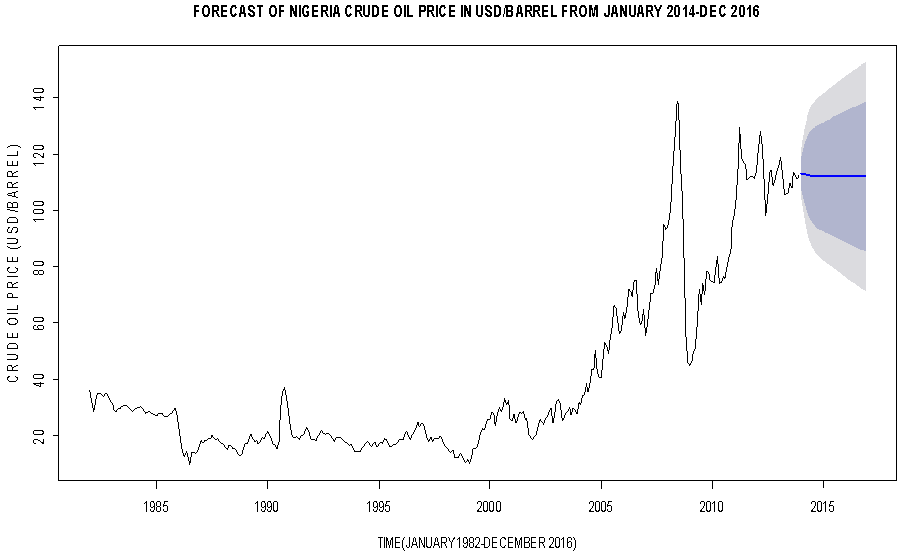 | Figure 6. The 80% (Heavy shaded band region) and 95% (Light shaded band region) confidence bands for the forecast crude oil price in USD/Barrel |
References
| [1] | www.nnpcgroup.com/nnpcbusiness/upstreamventures/oilproduction.aspx |
| [2] | L. Yu, S. Wang, and K. K. Lai, Forecasting crude oil price with an EMD-based neural network ensemble learning paradigm, Energy Economics, vol. 30, no. 5, pp. 2623–2635, 2008. |
| [3] | Y. Wei, Y. Wang, and D. Huang, Forecasting crude oil market volatility: further evidence using GARCH-class models, Energy Economics, vol. 32, no. 6, pp. 1477–1484, 2010. |
| [4] | C.C. Jesus, J. Adusei, and K. Sohbet, Modelling and Forecasting Oil Prices: The Role of Asymmetric Cycles, The Energy Journal, vol. 30, no. 3,pp. 81-90, 2009. |
| [5] | A. Shabri and R. Samsudin, Crude Oil Price Forecasting based on Hybridizing Wavelet Multiple Linear Regression Model, Particle Swarm Optimization Techniques and Principal Component Analysis, The Scientific World Journal, vol.2014, Article ID 854520 |
| [6] | www.cenbankorg/rates/crudeoil |
| [7] | M. R .Spiegel and L. J. Stephens, Schaum’s Outline of Theory and Problems of Statistics, third edition (McGrow- Hill, 1999). |
| [8] | G.E.P. Box and G.M. Jenkins, Time series analysis, forecasting and control, 2nd ed. (Holden-Day, San Francisco, 1976). |
| [9] | A. Pankratz, Forecasting with Univariate Box-Jenkins Models: Concepts and Cases (Wiley series in Probability and Mathematical Statistics, 1983). |
| [10] | R Development Core Team R: A language and environment for statistical computing// R Foundation for statistical computing. Vienna, Austria: 2014. 3-900051-07-0. |
| [11] | G. M. Ljung and G. E. P. Box , On a Measure of Lack of Fit in Time Series Models, Biometrika, vol. 65, pp. 297 ,1978. |
| [12] | D. A. Dickey and W.A .Fuller, Autoregressive Time Series with a Unit Root, Journal of American Statistical Association, vol.74, pp.427-431, 1979. |
| [13] | H. Akaike, A New Look at the Statistical Model Identification, IEEE Trans. Automat. Contr.) Ac-19, 1974, 716-723. |
| [14] | G. Schwarz, Estimating the Dimension of a Model, Annals of Statistics, 6,1978, 461-464. |

 denote a non-stationary time series which could adequately be modelled by the ARIMA (p,d,q) model defined by:
 denote the order of the AR part of the model,
  denote the order of the MA part of the model and
  denote the number of times the non-stationary time series need to be differenced to make it stationary. Interestingly, when
 , (1) reduces to a stationary ARMA (p,q) process defined by:
 and
and  are as defined above.
 depends on the immediate past of the process and
  is essentially a stationary white noise process i.e.
  Applying the first differencing to (3) we have:
 is a white noise process and stationary.
 . The ACF plot of the MA process shows cut-off to zero after lag
  while its PACF decays exponentially to zero. The combination of the AR (P) and the MA (q) processes is known as the ARMA (p,q) process (Equation 2) which has ACF and PACF that decays exponentially to zero. The maximum likelihood estimation method could be used in the estimation stage to estimate the parameters of the identified model(s). The last stage (diagnostic checking) involves assessing the validity of the identified and fitted models through possible statistically significant test. Finally, the best fitting ARIMA model would be used to make forecast.
 denote the time series of Nigeria crude oil price in USD (January 1982 - December 2013). We present the time series plot, ACF plot and the PACF plot of the crude oil price data as follows:From the time series plot (Top panel) of Nigeria crude oil price in USD/Barrel in Figure 1, it could be seen that the series shows an overall fluctuation. It also appears to be relatively stable from January 1982 to about the first Quarter of 2000 where a substantial upward trend followed immediately; and thereafter a sharp fall at about the last Quarter of 2008, followed by a price increase at about the first Quarter of 2009 which persisted until December 2013. The presence of trend in the series suggests a non constant mean over time. The ACF plot (Centre panel) decays very slowly to zero where these observations from the time series plot and the ACF plot imply a non-stationary time series. The PACF plot (Bottom panel) has a cut-off at lag 1 suggesting an AR(1)
  model for the crude oil price data. Although, the crude oil price data has through the above visual inspection shown non-stationarity, an AR (1) model is fitted to the data as suggested by the PACF.
 Hence, the diagnostic plots in Figure 2.
 model on the basis of the standardized residuals
 where these observations imply that the standardised residuals are correlated hence, not normally distributed. Consequently, a test (the Augmented Dickey-Fuller test [12]) to further substantiate the suggestive non-stationarity that is based on the subjective visual display of the time series plot is carried out in section 3.2.
 or
or  Presented in Figure 3 are the time series plot, ACF plot and the PACF plot of the first ordinary difference of the crude oil price data.


 or
or
 model for the crude oil price data. From the information presented in Table 4, we could see that the following model parameters:
  of the fitted ARIMA (6,1,7) model are redundant (not statistically significant) due to their associated standard errors which are more than two times larger than the estimated model parameters. Hence the diagnostic plots are as follows:

 . Clearly, in support of the ACF plot. However, the redundancy of a large number of the fitted model parameters would undermine the adequacy of the fitted ARIMA (6,1,7) model. But since
  and
and  are the only statistically significant parameters of the model it therefore suggests that the ARIMA (2,1,2) be fitted to the crude oil price data leading to a reduced and parsimonious model.Clearly, from Table 5 all the model parameters are statistically significantly different from zero as suggested by the small standard errors corresponding to the ARIMA (2,1,2) parameters. The diagnostic plots are immediately presented in Figure 5.


 Abstract
 Reference
 Full-Text PDF
 Full-text HTML

 model fitting


 model fitting
 Model fitting