1. Introduction

The statistical process control helps managers understand, monitor and continuously improve the quality of products and services. In the 1930s, Shewhart [1] created the control charts to monitor processes, and then recognized the need to monitor processes considering the multivariate control.

The traditional control charts assume by means of hypothesis independence among observations of variable that one wishes to monitor. However, high production speeds generate correlation among the quality characteristics and dependence among observations of one quality characteristic of neighbor products according to the manufacturing instant [2]. Some studies were done in order to evaluate the charts performance of multivariate control in autocorrelation presence, concluding that there is a drop in these charts performance [3-6].

The multivariate processes monitoring whose observations are autocorrelated appears in recent publications. Mastrangelo and Forrest [7] have made available a program to generate autocorrelated data where it is possible to simulate displacement in value of average of variable under monitoring. Pan and Jarrett [8] proposed the use of waste of the VAR(p) model to monitor autocorrelated processes. The technique requires fitting the model to process data for later use of waste in the T² chart. Arkat [5] makes use of artificial neural networks for monitoringmultivariate autocorrelated processes. Issam and Mohamad [6] propose the use of the SVR (support vector regression) method to monitor changes in the mean vector in autocorrelated processes through the MCUSUM control chart. Hwarng and Wang [9] established the use of neural networks that are able to identify shifts in the mean vector of autocorrelated processes. There are several other works on monitoring autocorrelated processes [10-13].

Autocorrelation compromises the use of control chart, for false alarms increase when it is disregarded, that is, when the control limits are established under hypothesis of autocorrelation absence [7, 14-16].

Kalgonda and Kulkarni [3] proposed the Z chart to monitor two or more quality characteristics for comments which follow a VAR(1) model. The advantage of Z chart in relation to T² chart is that it identifies the quality characteristic that suffers change in its average value. The authors present an empirical procedure to determine the control limit (CL) of Z chart. They assume that there is a correlation between the observations of X and Y and there is dependency in the time between X and Y observations and this correlation and autocorrelation structure is of a VAR(1) model. This article shows that for this correlation and autocorrelation structure there is a linear relationship between the CL of Z chart and variances and matrix covariance of cross-covariance of X and Y. For a wide range of values of cross-correlation and autocorrelations, it was obtained is a coefficient for determining the linear relationship model higher than 0.95.

This article aims to present a linear regression model to obtain the control limit of the Z chart that ensures the false alarm rate desired for a wide range of values of cross correlations and autocorrelations. The only method described in the literature for obtaining the CL was the Kalgonda and Kulkarni method [3] which, besides complicated, almost always gives control limits more spaced than it is necessary to meet the desired false alarm rate.

The paper is organized as follows: it is presented, in section 2, the model that describes the quality characteristics of a process with cross-correlations and autocorrelations; in section 3, the Z control chart; section 4 presents the regression model for obtaining the CL of Z chart and compares the false alarm rate calculated using the limits obtained by regression with the false alarm rate calculated using the limits obtained by the method of Kalgonda and Kulkarni [3].

2. Model Describing the Quality Characteristics

The classical control procedures in multivariate processes consider the basic assumption that observations follow a multivariate normal distribution and are independent with vector of means and the variance-covariance matrix.

(1)

where represents observations by a vector of order (p is the number of variables); are independent random vectors of order with multivariate normal distribution whose mean is zero and variance-covariance matrix .

The independence assumption is violated in many manufacturing processes, which makes equation (1) inadequate to represent such observations. Vector of auto regression of first-order, or VAR(1), equation (2), have been used to model multivariate processes with temporal correlation among observations of a variable and correlation among observations of different quality characteristics [2-6, 9, 17-20].

In multivariate autocorrelated processes, the VAR(1) model is represented as follows:

(2)

where is the data vector of order ; is the mean vector of order and is a matrix containing autoregressive parameters of order p x p and are independent random vectors of order with multivariate normal distribution whose mean is zero and variance-covariance matrix.

If is a zero matrix, equation (2) is reduced to equation (1), that is, one has the classical model for independent data over the time. Otherwise, the data will be dependent over the time and the model variation structure is represented by the cross-covariance matrix given by equation (3) [21].

Under the assumption that the process is stationary, for all t, cross-covariance matrix will be:

(3)

Being stationary means that is constant for all and the cross-covariance matrix does not depend on t, it depends only on h which represents the interval over the time and between the vector and.

The matrix is formed by the elements given by:

(4)

Since the cross-covariance matrix originally depends on the measurement unit of involved variables, sometimes its interpretation is not simple. A more convenient way to evaluate the relationship of variables in the process is given by using the cross-correlation matrix:

(5)

where D is the diagonal matrix formed by the elements, for all i=j, of matrix .

The cross-covariance matrix for h=0, , when and are known, can be obtained by the ratio of Yule-Walker [24]:

(6)

Assuming is a data vector with p-varied distribution and follow the model described in equation (2), according to Kalgonda and Kulkarni [3] and Kalgonda [20],

(7)

If the process is in statistical control, follows a multivariate normal distribution with mean vector and cross-covariance matrix .

3. Z Control Chart

With the simultaneous use of X charts to control two or more quality characteristics, it is possible to identify which of them has been affected by the special cause. However, when the variables are dependent or correlated, to obtain the control limits of the X charts is no longer trivial [22], for the probability that the values of X₁, X₂, ... , X_p, are within the control limits is no more given by:

(8)

where p is the number of variables and the probability of a false alarm.

Kalgonda and Kulkarni [3] proposed a control chart called a Z chart for monitoring the mean vector of multivariate autocorrelated procedures. The chart maintains the overall error and allows the variables identification whose means have changed with the emergence of a special cause. The authors adapted the statistical control technique of means vector for independent observations proposed by Hayter and Tsui [25] and considered that autocorrelation in the process follows the VAR(1) model.

At t time instant, the monitoring statistics of Z chart is given by , where:

(9)

where is the value of the i-th variable at instant of time t and is the i-th diagonal element of the cross covariance matrix to h=0.

For a certainvalue, the CL of the Z chart is given by:

(10)

The process is considered in statistical control if ≤ LC. Otherwise, there is evidence that the mean of at least one of the p variables changed.

The distribution of statistic is not known; Kalgonda and Kulkarni [3] obtained the CL by simulation following the steps:

− Step 1. Generating a large number of vectors (N = 10000) with observations according to the standard p-variate model;

− Step 2: Calculating the statistic for each of the N vectors generated in step 1;

− Step 3 Obtaining the empirical distribution of the statistic, find the separatrix of order (1−) and assign this value to the CL.

The steps described by Kalgonda and Kulkarni [3] almost always lead to control limits more widely spaced than necessary to meet the desired rate of false alarms (ARLo>). The ARLo is the average number of observations among false alarms. For independent and uncorrelated variables the ARLo = [23].

To illustrate, let it be the bivariate case (p=2):

; and , then from (6) it has been obtained the cross-covariance matrix,

(11)

The method proposed by Kalgonda and Kulkarni [3] provides for a CL of 3.0191. For CL = 3.0191, it has been obtained by simulation one ARLo = 261.78. The appendix provides details of simulation.

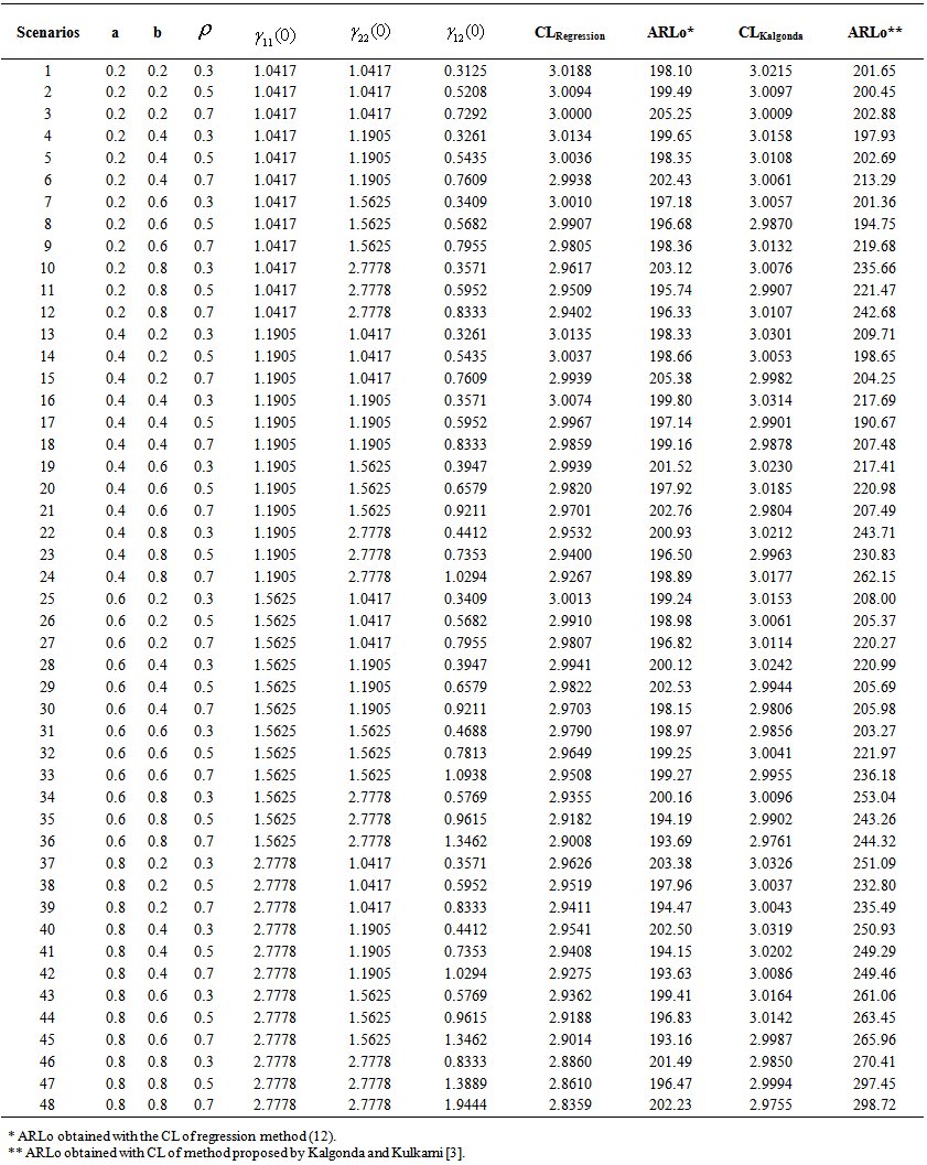
Because of autocorrelation ARLo does not follow a geometrical distribution, for the probability of false alarm is not constant. Depending on the parameters of the VAR(1) Model, the CL of Z chart provided by the method of Kalgonda and Kulkarni [3] leads to different ARLos. In order to solve this problem, this paper proposes a linear regression model which provides the CL of Z chart corresponding to the desired ARLo (see Figure 1 of section 4).

4. Proposed Method

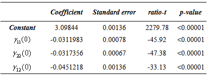
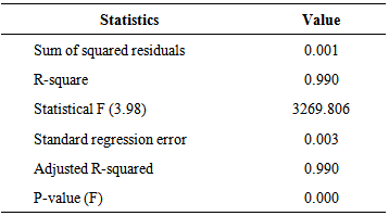
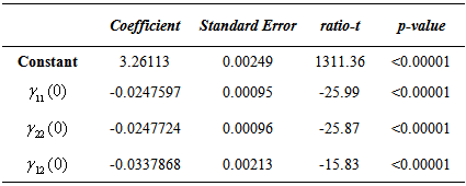
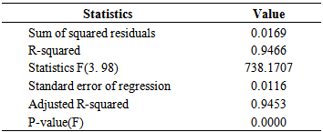
In order to facilitate the use of the Z chart, the CL values were obtained by simulation for a wide range of parameter values of autocorrelation matrix and of the covariance matrix of bivariate VAR(1) error. Two regression models were made, one for ARLo of 200 and another for ARLo of 370. In regression models estimation, the CL values were allocated to the dependent variable vector and the elements values of cross-covariance matrix were allocated to the independent vectors matrix. The model fitted to the data providing R² values very close to 1, see Tables 2 and 4. Model parameters for ARLo of 200 and 370 are shown in Tables 1 and 3, respectively.

Table 1. Parameters of regression model - ARLo = 200

Table 2. Statistics of the model in Table 1

With the values of , andof cross-covariance matrix it is possible to obtain the control limits of the Z chart.

For ARLo=200:

(12)

For ARLo=370:

(13)

It has also been considered the case where the ARLo is equal to 370. The results of regression model are shown in Tables 3 and 4.

Table 3. Regression model parameters - ARLo = 370

Table 4. Statistics of model in Table 3

4.1. Sensitivity Analysis of the Proposed Method

To illustrate the use of the proposed method and its diagnosticability in the presence of autocorrelation, one considers a similar case of bivariate vector as presented in Kalgonda and Kulkarni [3]. The results in Figure 1 illustrate the ability of the proposed method to evaluate the CL. One considers the following scenarios to carry out the analysis:

ARLo is equal to 200, it has been adopted values a and b of matrix ranging from0.2 to 0.8 and values of the matrix equal to 0.3, 0.5 and 0.7. In practice these values are unknown; the elements of the cross-covariance matrix that depend on a, b and are estimated according to equation (6). It is important to notice that an interesting subject of research is the study of Z chart in multivariate process.

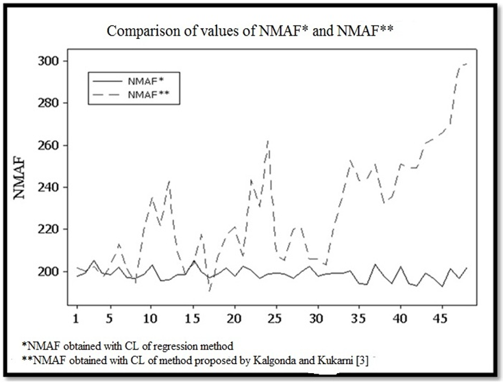Figure 1. NMAF = ARLo obtained by regression and Kalgonda method [20]

The ARLo values for 48 different scenarios are presented in Table B1 of Appendix B and were used in the construction of Figure 1.

From Table B1 and Figure 1, it is observed that the regression model in order to obtain the CL is better than the Kalgonda and Kulkarni method [3], for it keeps the ARLo always close to 200 for all scenarios.

5. Conclusions

This paper has presented a method better than the one proposed by Kalgonda and Kulkarni [3] for obtaining the CL of Z chart. Better in order to provide control limits that lead to false alarms rates closer to those desired. The method of Kalgonda and Kulkarni [3] provides generally CL values larger than the one necessary; this excessive protection against false alarms occurrence reduces the control chart ability to detect changes in the process. The method proposed in this article requires great effort for the construction of the linear regression model; however, after obtaining it, the calculation of CL of Z chart is immediate.

Appendix A – Method Used in Simulation of Multivariate Temporal Series with Generation Process VAR(1)

Simulation of a multivariate temporal series with p dimension and T size:

1) It is created errors with Gaussian multivariate distribution of order p, , by means of multiplication of matrix P of order (p x p) with vector V = (v₁ , ... , v_p) of order (px1), where and V ~ N(0,1).

(A1)

For instance, if p=2:

(A2)

1) The step 1 is repeated T times for generation of a sort of errors.

2) With values, it is obtained X_t in a recursive way by equation A3 turning t=1,2.....,T.

(A3)

where: X_t is a matrix of order( px 1); is a mean matrix of order(p x 1); is the autocorrelation matrix of order(p x p).

3) With vector generated in (3), it is obtained the statistics.

4) The CL of Z chart is calculated by a binary search until the ARLo is equal to the desired value.

Appendix B –ARLo values

Table B1. Comparison of ARLo values based on regression model and on Kalgonda and Kulkarni method [3]