1. Introduction

In ohmically heated (lowβ) tokamaks, radial pressure balance is achieved by the poloidal field, and toroidal force balance is achieved by equality between the external vertical field force (Lorentz force) and outward forces due to toroidal configuration. But, in toroidal force balance problem, the two opposite forces may be not equal and therefore plasma intend to shift inward or outward, which it is dangerous for tokamak plasma. Therefore, plasma equilibrium study is one of the fundamental problems of the magnetically confined plasmas. There are many available experimental methods and analytical solutions of the steady statemagnetohydrodynamics (MHD) equations, in particular, the Grad-Shafranov equation for the plasma equilibrium problem. Control of plasma position has important role in plasma confinement and to achieve optimized tokamak plasma operation. Determination of accurate plasma position during confinement time is essential to transport it to a control system based on feedback. Over the years different methods have been developed to analysis the tokamak plasma equilibrium problems [1-54].

In this paper we present two experimental and analytical methods for determination of plasma column center in IR-T1 Tokamak, which it is a small, air core, low β and large aspect ratio tokamak with a circular cross section (see Table 1). Details of the poloidal flux loops technique for determination of Shafranov Shift will present in section 2. Analytical solution of the Grad-Shafranov equation will present in section 3. Experimental results and comparative between them also will present in section 4. Summary and conclusion will present in section 5.

2. Poloidal Flux Loops Method in Measurement of Plasma Position

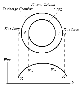
Poloidal flux loop is a simple toroidally loop which measure the poloidal magnetic flux and usually array of them use in control and reconstruction of plasma equilibrium states. The magnetic flux passing through such a loop is equal to, where represent to magnetic poloidal flux. In the ohmically heated tokamaks, ohmic coils field is the main fraction of poloidal flux which passing through the flux loop. Therefore to obtain net poloidal flux due to plasma, compensation will require for all excessive flux. Because of large area of the flux loop, the inductive voltage is also large and then it consists of usually one turn. According to relation for frequency response, it is obvious that because of small self inductance, frequency response of flux loop usually is higher than which desired.

Although magnetic probe suitable for measurement of plasma position only in circular cross section plasma and not for elongated one, but the flux loop either in elongated and or circular cross section tokamaks can be used. Therefore we used these two techniques for the IR-T1 tokamak with circular cross section.

The plasma boundary is usually defined by Last Closed Flux Surface (LCFS). In the LCFS poloidal magnetic flux is constant, if we install some flux loops at some distance in vicinity of LCFS, then we can find plasma displacement from difference in poloidal fluxes that received with flux loops according to Shafranov equation. In the quasi-cylindrical coordinates for the poloidal magnetic flux we have [1].

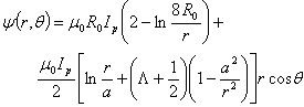where

(1)

and where 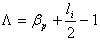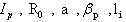are the plasma current, major and minor plasma radiuses, poloidal beta and internal inductance of the plasma. The relationship between poloidal magnetic flux and plasma displacement is:

(2)

According to Figure (1) the poloidal flux is obtained:

(3)

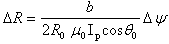
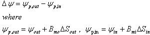
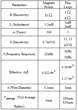
and where and are the poloidal flux which obtained with outer and inner flux loops, and are the average magnetic fields between outer and inner flux loops and the plasma surface respectively which can be obtained from magnetic probe, is the intervening area for each loop defined as: which d is distance between LCFS and each loop and is the distance between the midpoint (d/2) and center of the facility.

In the IR-T1 tokamak two poloidal flux loops designed and installed on outer surface of vacuum chamber in polar angles and , with radiuses and (see Figure (1) and Table (2)).

Table 1. Parameters of the IR-T1 tokamak

Table 2. Design parameters of the poloidal flux loops and magnetic probes

Figure 1. Schematic diagrams for positions of the two flux loops on outer surface of IR-T1 tokamak

As mentioned above, the ohmic field is the significant fraction of the poloidal flux which passing through the flux loop, therefore essentially compensation is needed. Compensation is done with all fields discharge without plasma and subtraction them from the total flux that received with flux loop. Experimental result for measurement of plasma position using this method will present in section 4.

3. Analytical Solution of the Grad-Shafranov Equation

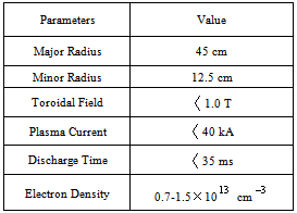
For axially symmetric configurations, Maxwell's equations together with the force balance equation from MHD equations, for stationary and ideally conducting plasmas, reduce to the two-dimensional, nonlinear, elliptic partial differential equation, or Grad-Shafranov equation (GSE) [1]. In some of the work, authors solved the Grad-Shafranov equation by expanding the free functions (, and ) in different order in (flux function). In this section, we regarded quadratic order (which proposed by Guazzotto [3]), and examined on the IR-T1.

The GSE is:

(4)

where

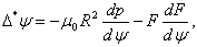
If we choose the free functions to be quadratic in as [3]:

(5)

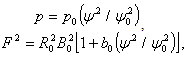
where are the values of , p, and F on magnetic surfaces axis, is the major radius, and is the vacuum toroidal field.

The Grad-Shafranov equation reduces to:

(6)

where .

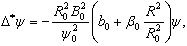
With normalizing variables as , and , Eq. (6) can then be written as:

(7)

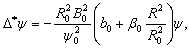
where, is the inverse aspect ratio, and

(8)

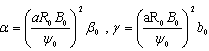
The solution of Eq. (7) in cylindrical coordinates can be written as:

(9)

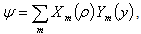
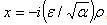where , and for up-down symmetric case, obtained as:

(10)

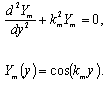
Also can be written as:

(11)

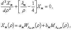
where , , and are the Whittaker functions, and in this model .

Guazzotto proposed only three terms for m, and then can be written as:

(12)

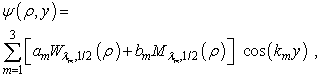
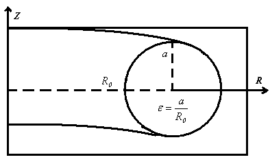
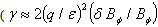
where , , and are nine unknown coefficients which must be determined. The first six of them can be obtained from boundary conditions. The boundary conditions for the points of inner, outer, and top of the plasma cross section are (see Figure (2)):

(13)

and condition for right convexity on the inboard midplane is:

(14)

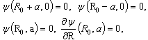
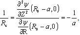
also two conditions, one defining the location of the magnetic axis () and the other the normalization for on magnetic axis:

(15)

Figure 2. geometry used for the boundary conditions

These are seven boundary conditions for seven unknown coefficients ().

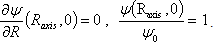
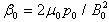
But for other three coefficients, by setting (the simplest solution for GSE independent of Z), and introduce one approximate value for the (, negative for diamagnetism plasma), and assuming that be imaginary and be real, the values of can be determined by minimizing the error function between traditional plasma shape (), and analytical plasma shape. Appropriate error function between them defined as follow:

(16)

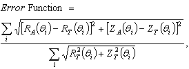
where subscripts (A and T) indicates the analytical and traditional plasma shape parameters respectively, and sum in minimum include 3 angles () for our purpose (circular plasma).

In general by minimizing the error function (e.g. by Mathematica) as possible to zero, and finding optimal values for , and also solving seven equations for the boundary conditions (Eqs. (13), (14), (15)), six unknown coefficients (), moreover can be find. Therefore the magnetic flux surfaces can be plot by substituting these nine coefficients and also input parameters as , and in Eq. (12). Moreover the Shafranov shift (), is also can be obtained by subtracting from. We repeat 18 times this procedure for different approximate values for during time interval of target shot (for example the magnetic flux surfaces at t=15ms correspond to shown in Figure (3)), and obtaining time interval of Shafranov shift. Results were shown in Figure (4).

4. Experimental Results and Comparison Between Them

For determination of the plasma position using the first method, we needed for determination of the poloidal magnetic flux around the plasma. Therefore we designed and installed two poloidal flux loops on outer surface of the IR-T1 chamber. Positions of the flux loops were shown in figure (1). Also, plasma current and average vertical field, were obtained from the Rogowski coil and magnetic probe, respectively.

According to the Faraday’s law, output of all magnetic diagnostics proportional to derivative of the magnetic flux which passing through them, therefore we needed to integrate the output of the flux loops and magnetic probes after compensating their output.

The integrator output is given by:

(17)

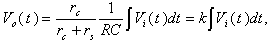
where RC is the integrator time constant, and where is the inductive voltage supplied by the flux loops and each one of the magnetic probes, which were placed around the IR-T1 tokamak vacuum chamber.

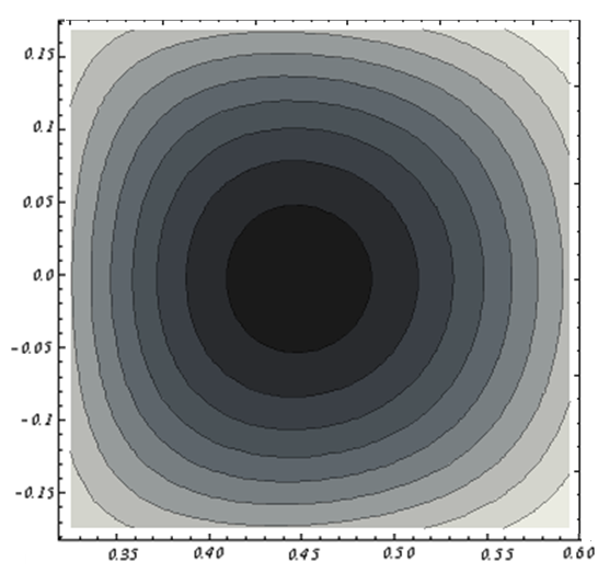
Figure 3. Magnetic Flux Surfaces obtained by the Second Analytical Method at t=15ms in Target Shot correspond to on IR-T1 Tokamak, Displacement of the Plasma Column Center observable

Figure 4. Horizontal Displacement (H.D.), determined by the (c) Flux loop and (b) Analytical methods along the (a) plasma current

We used the two methods to determine the horizontal displacement in IR-T1 as shown in Figure (4). These figures show that two methods give us a same horizontal displacement. Moreover we plot the magnetic flux surfaces or Eq. (12) for plasma parameters at t=15ms in target shot on IR-T1 tokamak, as we expect there is displacement of plasma column center as shown in Figure (3).

5. Summary and Conclusions

In this paper we determined the Shafranov shift by two experimental and analytical methods in IR-T1 tokamak. In the first method we designed and installed two poloidal flux loops on the outer surface of the IR-T1 tokamak chamber, and then plasma displacement determined from them. 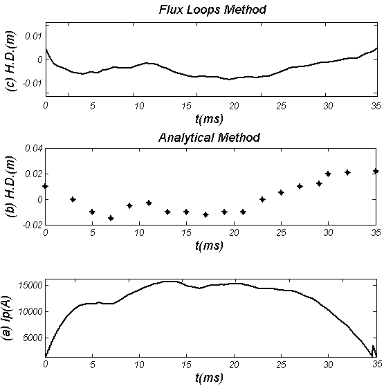To compare the plasma position obtained using this method, the analytical solution of the Grad-Shafranov equation based on expanding of the free functions, quadratic in is also presented, and experimented on IR-T1. Results show that two methods are in good agreement with each other. The acceptable differences between them are because of (1) approximation in measurement of poloidal flux on LCFS, (2) the approximate values chosen for, and (3) the errors do not become zero during minimizing the error function.