Ranjit R. Dhunde1, G. L. Waghmare2
1Department of Mathematics, Datta Meghe Institute of Engineering Technology and Research, Wardha, M.S., India
2Department of Mathematics, Government Science College, Gadchiroli, M.S., India
Correspondence to: Ranjit R. Dhunde, Department of Mathematics, Datta Meghe Institute of Engineering Technology and Research, Wardha, M.S., India.
| Email: |  |
Copyright © 2017 Scientific & Academic Publishing. All Rights Reserved.
This work is licensed under the Creative Commons Attribution International License (CC BY).
http://creativecommons.org/licenses/by/4.0/

Abstract
Double Laplace transform method has not received much attention unlike other methods. This article presents its effectiveness while finding the solutions of wide classes of equations of mathematical physics.
Keywords:
Double Laplace transform, Single Laplace transform, Partial differential equations
Cite this paper: Ranjit R. Dhunde, G. L. Waghmare, Double Laplace Transform Method in Mathematical Physics, International Journal of Theoretical and Mathematical Physics, Vol. 7 No. 1, 2017, pp. 14-20. doi: 10.5923/j.ijtmp.20170701.04.
1. Introduction
In recent years, Eltayeb and Kilicman [1-3] applied double Laplace transform (DLT) to solve wave, Laplace’s and heat equations with convolution terms, general linear telegraph and partial integro-differential equations. In 2016, L. Debnath [4] discussed the properties and convolution theorem of DLT, and applied it to functional, integral and partial differential equations. Further, Ranjit Dhunde and G. L. Waghmare in [5] applied double Laplace transform technique for solving linear partial integro-differential equations with a convolution kernel.Analogous to [6], we consider linear, one-dimensional, time-dependent partial differential equation (PDE) of the form | (1.1) |
where  are given coefficients and N, M are positive integers and
  is the source term. Associated with (1.1), we can consider the initial conditions
  | (1.2) |
and boundary conditions | (1.3) |
Further, we assume that the functions 
 are such that problems (1.1), (1.2) and (1.3) have a solution.The main objective of this paper is to develop new applications of the double Laplace transform for solving linear PDE’s of the type (1.1) subject to the initial conditions (1.2) and boundary conditions (1.3).A wide range of linear PDE’s are considered which include the advection-diffusion equation (Section 4.1), the reaction-diffusion equation (Section 4.2), the telegraph equation (Section 4.3), the Klein-Gordon equation (Section 4.4), the dissipative wave equation (Section 4.5), the Korteweg-de Vries (KdV) equation (Section 4.6) and the Euler-Bernoulli equation (Section 4.7).
2. A Brief Introduction to Double Laplace Transforms
Let  be a function of two variables x and t defined in the positive quadrant of the xt-plane. The double Laplace transform of the function
  as given by Ian N. Sneddon [7] is defined by
  | (2.1) |
whenever that integral exist. Here p and s are complex numbers.From this definition we deduce | (2.2) |
The double Laplace transform formulas for the partial derivatives of an arbitrary integer order are | (2.3) |
 | (2.4) |
The inverse double Laplace transform 
 is defined as in [4] by the complex double integral formula
 | (2.5) |
where  must be an analytic function for all p and s in the region defined by the inequalities
 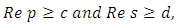 where c and d are real constants to be chosen suitably.
3. Double Laplace Transforms Method
Applying the double Laplace transform on both sides of (1.1), we get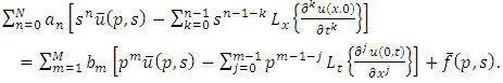 | (3.1) |
Further, applying single Laplace transform to initial (1.2) and boundary conditions (1.3), we get | (3.2) |
By substituting (3.2) in (3.1) and simplifying, we obtain | (3.3) |
Equation (3.3) is an algebraic equation in  Solving this algebraic equation and taking in verse double Laplace transform of
  we get an exact solution
  of (1.1).
4. Applications
In this section, we apply double Laplace transform (DLT) method to linear partial differential equations.
4.1. The Advection-Diffusion Equation
Taking 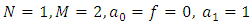 in (1.1), we obtain the advection-diffusion equation
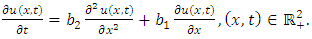 | (4.1) |
It governs the release of hormones from secretory cells in response to a stimulus in a medium, flowing past the cells and through a diffusion column, also the dispersion of pollutants in rivers [6].If (4.1) is solved subject to the initial condition 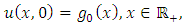 | (4.2) |
and the boundary conditions 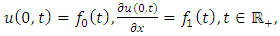 | (4.3) |
then (3.3) gives the solution of (4.1),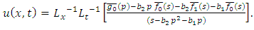 | (4.4) |
Example 4.1: Taking  then (4.1) becomes
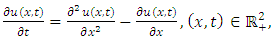 | (4.5) |
and consider the initial and boundary conditions | (4.6) |
 | (4.7) |
Substituting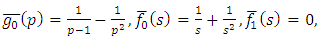 | (4.8) |
in (4.4), we get solution of (4.5)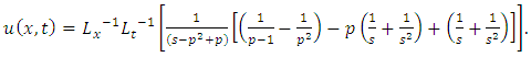 | (4.9) |
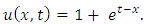
Simplifying, we obtain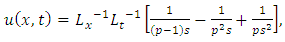 | (4.10) |
 | (4.11) |
4.2. The Reaction-Diffusion Equation
Taking  in (1.1), we get the reaction-diffusion equation
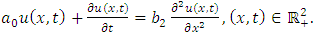 | (4.12) |
If (4.12) is solved subject to the initial condition (4.2) and boundary conditions (4.3) then (3.3) gives the solution of (4.12),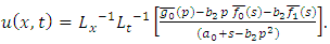 | (4.13) |
4.2.1. The Heat (Diffusion) Equation
Taking  in (4.12), we obtain the linear heat equation
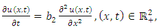 | (4.14) |
where  is the constant coefficient of diffusion.If (4.14) is solved subject to the initial condition (4.2) and boundary conditions (4.3) then (4.13) gives the solution of (4.14),
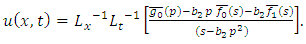 | (4.15) |
4.3. The Telegraph Equation
Taking 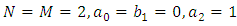 in (1.1), we obtain the linear telegraph equation
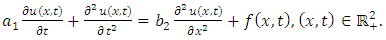 | (4.16) |
The telegraph equation is used in signal analysis for transmission and propagation of electrical signal and also modelling reaction diffusion.If (4.16) is solved subject to the initial conditions 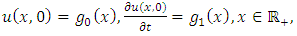 | (4.17) |
and boundary conditions (4.3) then (3.3) gives the solution of (4.16), | (4.18) |
Example 4.2: Take  in (4.16) to yield
 | (4.19) |
and consider the initial and boundary conditions | (4.20) |
 | (4.21) |
Substituting | (4.22) |
in (4.18), we get  | (4.23) |
Simplifying, we obtain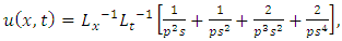 | (4.24) |
 | (4.25) |
4.3.1. The Wave Equation
Substituting  in (4.16), we obtain wave equation
 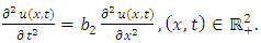 | (4.26) |
If (4.26) is solved subject to the initial conditions (4.17) and boundary conditions (4.3) then (4.18) gives the solution of (4.26),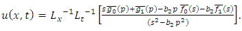 | (4.27) |
4.4. The Klein-Gordon Equation
Taking  in (1.1), we obtain the Klein-Gordon equation
 | (4.28) |
The Klein-Gordon equation plays an important role in the study of solutions in condensed matter physics, quantum mechanics and relativistic physics.If (4.28) is solved subject to the initial conditions (4.17) and boundary conditions (4.3) then (3.3) gives the solution of (4.28),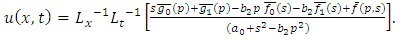 | (4.29) |
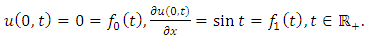
Example 4.3: Take 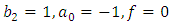 in (4.28) to yield
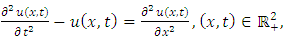 | (4.30) |
and consider the initial and boundary conditions | (4.31) |
 | (4.32) |
Substituting | (4.33) |
in (4.29), we get solution of (4.30)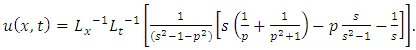 | (4.34) |
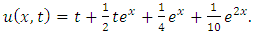
Simplifying, we obtain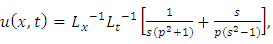 | (4.35) |
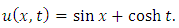 | (4.36) |
Example 4.4: Take  in (4.28) to yield
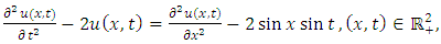 | (4.37) |
and consider the initial and boundary conditions | (4.38) |
 | (4.39) |
Substituting | (4.40) |
in (4.29), we get solution of (4.37)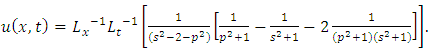 | (4.41) |
Simplifying, we obtain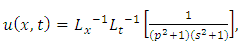 | (4.42) |
 | (4.43) |
4.5. The Linear Dissipative Wave Equation
Substituting  in (1.1), we obtain the linear dissipative wave equation
 | (4.45) |
If (4.45) is solved subject to the initial conditions (4.17) and boundary conditions (4.3) then (3.3) gives the solution of (4.45), | (4.46) |
Example 4.5: Take  in (4.45) to yield
 | (4.47) |
and consider the initial and boundary conditions | (4.48) |
 | (4.49) |
Substituting | (4.50) |
in (4.46), we get solution of (4.47) | (4.51) |
Simplifying, we obtain | (4.52) |
 | (4.53) |
4.6. The Korteweg-de Vries (KdV) Equation
Substituting  in (1.1), we obtain the linear Korteweg-de Vries (KdV) equation
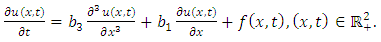 | (4.54) |
It governs long water waves, in water of relatively shallow, for very small amplitudes [6]. When  (4.54) represents a third-order dispersive equation.If (4.54) is solved subject to the initial condition (4.2) and boundary conditions
 | (4.55) |
then (3.3) gives the solution of (4.54), | (4.56) |
Example 4.6: Taking 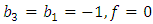 then (4.54) becomes
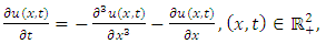 | (4.57) |
and consider the initial and boundary conditions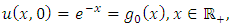 | (4.58) |
 | (4.59) |
Substituting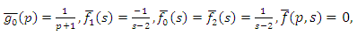 | (4.60) |
in (4.56), we get solution of (4.57) | (4.61) |
Simplifying, we obtain | (4.62) |
 | (4.63) |
Example 4.7: Taking  in (4.54) to obtain the linear third-order dispersive, inhomogeneous equation
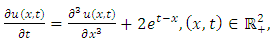 | (4.64) |
and consider the initial and boundary conditions | (4.65) |
 | (4.66) |
Substituting | (4.67) |
in (4.56), we get solution of (4.64) | (4.68) |
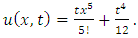
Simplifying, we obtain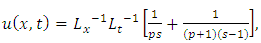 | (4.69) |
 | (4.70) |
Example 4.8: Taking  in (4.54) to obtain
 | (4.71) |
and consider the initial and boundary conditions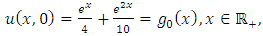 | (4.72) |
 | (4.73) |
Substituting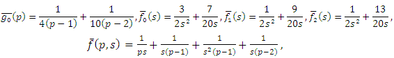 | (4.74) |
in (4.56), we get solution of (4.71)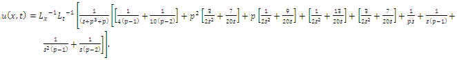 | (4.75) |
Simplifying, we obtain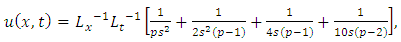 | (4.76) |
 | (4.77) |
4.7. The Euler-Bernoulli Equation
Taking  in (1.1), we obtain the Euler-Bernoulli equation
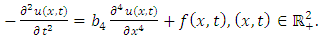 | (4.78) |
It governs the deflection of an elastic beam under the action of a load  In (4.78), the solution
  represents the deflection of the beam and
  is its flexural rigidity.If (4.78) is solved subject to the initial condition (4.17) and boundary conditions
 | (4.79) |
then (3.3) gives the solution of (4.78), | (4.80) |
Example 4.9: Take 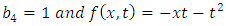 in (4.71) to yield
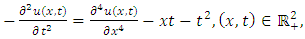 | (4.81) |
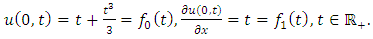
and consider the initial and boundary conditions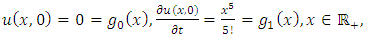 | (4.82) |
 | (4.83) |
Substituting | (4.84) |
in (4.80), we get solution of (4.81) | (4.85) |
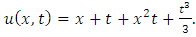
Simplifying, we obtain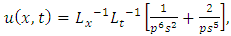 | (4.86) |
 | (4.87) |
5. Conclusions
The examples show that double Laplace transform method is a best alternative for handling many equations of Mathematical Physics.
References
| [1] | H. Eltayeb, A. Kilicman, A note on solutions of wave, Laplace’s and heat equations with convolution terms by using a double Laplace transform, Applied Mathematics Letters 21 (2008) 1324-1329. |
| [2] | A. Kilicman, H. Eltayeb, A note on defining singular integral as distribution and partial differential equations with convolution term, Mathematical and Computer Modelling 49 (2009) 327-336. |
| [3] | H. Eltayeb, A. Kilicman, A note on double Laplace transform and telegraphic equations, Abstract and Applied Analysis, Volume 2013. |
| [4] | L. Debnath, The double Laplace transforms and their properties with applications to Functional, Integral and Partial Differential Equations, Int. J. Appl. Comput. Math, 2016. |
| [5] | Ranjit R. Dhunde, G. L. Waghmare, Solving partial integro-differential equations using double Laplace transform method, American Journal of Computational and Applied Mathematics 2015, 5(1): 7-10. |
| [6] | D. Lesnic, The Decomposition method for Linear, one-dimensional, time-dependent partial differential equations, International Journal of Mathematics and Mathematical Sciences, Volume 2006, pp. 1-29. |
| [7] | Ian N. Sneddon, The use of integral transforms, Tata McGraw Hill Edition 1974. |

 Abstract
 Reference
 Full-Text PDF
 Full-text HTML