Acha Chigozie Kelechi
Department of Mathematics/Statistics,College of Natural and Applied Sciences, Michael Okpara University of Agriculture,
Correspondence to: Acha Chigozie Kelechi, Department of Mathematics/Statistics,College of Natural and Applied Sciences, Michael Okpara University of Agriculture,.
| Email: |  |
Copyright © 2012 Scientific & Academic Publishing. All Rights Reserved.
Abstract
This paper uses the regression analysis and principal component analysis (PCA) to examine the possibility of using few explanatory variables to explain the variation in the dependent variable. It applied regression analysis and principal component analysis (PCA) to assess the yield of turmeric, from National Root Crop Research Institute Umudike in Abia State, Nigeria. This was done by estimating the coefficients of the explanatory variables in the analysis. The explanatory variables involved in this analysis show a multiple relationship between them and the dependent variable. A correlation table was obtained from which the characteristic roots were extracted. Also, the orthonormal basis was used to establish the linearly independent relationships of the variables. The regression analysis shows in details the constant and the coefficients of the three explanatory variables. On the other hand the principal component analysis estimates the first principal component second principal component and both components accounted for 71.4 percent of the total variation. The regression analysis and principal component analysis (PCA) yielded good estimates, which leads to the structural coefficient of the regression model. The study shows that regression analysis and principal component analysis (PCA) use few explanatory variables to explain variations in a dependent variable and are therefore efficient tools for assessing turmeric yield depending on the set objective. But that PCA is more efficient since it uses fewer variables to achieve the same result.
Keywords:
Turmeric, Correlation, Descriptive statistics, Model, Variables, Principal component analysis, Regression
Cite this paper: Acha Chigozie Kelechi, Regression and Principal Component Analyses: a Comparison Using Few Regressors, American Journal of Mathematics and Statistics, Vol. 2 No. 1, 2012, pp. 1-5. doi: 10.5923/j.ajms.20120201.01.
1. Introduction
Turmeric, the plant from which the data for this study is obtained, comes from the root of Curcuma longa, a green plant in the ginger family. It is a rhizome and therefore has a tough brown skin and bright orange flesh. When not used fresh, the rhizomes are boiled for several hours and then dried in hot ovens, after which they are ground into a deep orange-yellow powder commonly used as a spice in curries,for example in South Asian and Middle Eastern cuisine. It is also used for dyeing, and to impart color to mustard condiments. Its active ingredient is curcumin and it has a distinctly earthy, slightly bitter, slightly hot peppery flavor and a mustardy smell. Ground turmeric comes from fingers which extend from the root (see http: //www.en.wikipedia. org/wiki/Turmeric). Turmeric yield will be considered as the dependent variable whereas the temperature, relative humidity and rainfall averages could be seen as response variables(X’s), there are various statistical techniques used in the estimation of the response variable from the explanatory variable. The major statistical tools for the estimation of the coefficients of the explanatory variables in this study are regression and principal component analyses. The other statistical tools applied are correlation, orthonormality, descriptive statistics, and plots or graphs. The regression analysis was first used in 1908 by Karl Pearsonwho also invented PCA in 1901. However, the general purpose of regression analysis is to learn more about the relationship between several independent variables and a dependent variable whereas the PCA is mostly used as a tool in exploratory data analysis and for making predictive models.
1.1. Objectives of Study
The major objective of this study is to compare the efficiency of PCA and regression analyses in predicting the response variable Y using few explanatory variables(X’s).In addition to this, the following secondary objectives are pursued;i. To assess the orthonormality of the explanatory variables.ii. To solve the problem of multi-colinearity in a multiple regression model.
2. Literature Review
Turmeric grows wild in the forests of South and Southeast Asia. It has become the key ingredient for many countries like Indian, Persian and Thai. Over thirty (30)varieties areknown to exist. Some of these are,Amalapuram, Armour, Dindigam, Erode, Krishna, Kodur, Vontimitra, P317, GL Purm I and II, RH2 and RH10. According to, Chan,et al. (2009) turmeric (Curcuma longa) is a rhizomatous herbaceous perennial plant of the ginger family, Zingiberaceae. It is native to tropical South Asia and needs temperatures between 20℃ and 30℃ and a considerable amount of annual rainfall to thrive (see http://www.ars-grin.gov).For the rapid and effective growth of Turmeric;● The soil must be enriched with organic minerals.● The plant must be exposed to maximum sunlight.● It should have regular supply of water but too much water may cause the roots to decay.● Extra nutrition can be added to the soil by using different kinds of fertilizers (Jagadeeswaran R. et al 2005; Dohroo , 2007).In this study, multiple regression and Principal components analyses will be employed to achieve the stated objectives. The termmultiple regressionwas first used by Pearson, 1908, it is used to learn more about the relationship between several independent variables and a dependent variable. While the Principal components analysis is a technique for finding a set of weighted linear composites of original variables such that each composite (a principal component) is uncorrelated with the others. It was originally devised by Pearson (1901) though it is more often attributed to Hotelling (1933) who proposed it independently. Principal component is a weighted linear composite of the original variables found by a matrix analysis technique called eigen-decomposition which produces eigenvalues, this represents the amount of variation accounted for by the composite and eigenvectors (which give the weights for the original variables) (see http://www.pcp-net.org/encyclopaedia/pca.html).According to Jolliffe (2002), Miranda and Bontempi (2008), several data decomposition techniques are available for this purpose; Principal Components Analysis (PCA) is among these techniques that reduces the data into two dimensions. The set of data or elements or numbers arranged in a table (matrix) as rows (row vector) or columns (column vectors) called vectors are being used. Moreover, since the Orthonormal basis is a set of vectors which forms a basis for a vector space and each of these basis vectors are normalized and they are orthogonal to each other. Axler (1997) observed that orthonormal sets are not especially significant on their own. However, Wang, et al (2005) confirmed that orthonormal sets display certain features that make them fundamental in exploring the notion of of certain operator on vector spaces. The PCA of a multivariate Gaussian distribution centered at (1, 3) with a standard deviation of 3 in roughly the (0.878, 0.478) direction and of 1 in the orthogonal direction (see http://en.wikipedia.org/wiki/ orthonormality).The vectors shown are the eigenvectors of the scaled by the square root of the corresponding eigenvalue, and shifted so their tails are at the mean.
3. Materials and Methods
The data for this work was collected from National Root Crop Research Institute, Umudike, Abia State, Nigeria. It shows the explanatory variables and dependent variable on Turmeric () from1996 to 2010. The statistical method include table of correlation coefficient to check if there are relationshipsamong the explanatory variables.Descriptive statistics is adopted to describe the features of the data whileorthonormality plot is used to overcome multi-collinearity and show trend or pattern of the explanatory variables.Finally, multiple regression and the principal components are used in turn to determine which of the explanatory variables account for the variations in the dependent variable.All the analyses were carried out using Eviews 7 software.
4. Analysis and Discussion of Results
Descriptive statistics for the set of data| Table 1. Descriptive statistics for the all the variables |
| | | YEAR | X1 | X2 | X3 | | Mean | 47.50467 | 27.22667 | 48.90667 | 61.00000 | | Median | 47.45000 | 27.40000 | 48.20000 | 61.00000 | | Maximum | 68.28000 | 29.40000 | 58.90000 | 69.00000 | | Minimum | 32.02000 | 23.50000 | 41.40000 | 52.00000 | | Std. Dev. | 10.68167 | 1.968127 | 6.366594 | 5.398412 | | Skewness | 0.227370 | -0.508894 | 0.262600 | -0.039476 | | Kurtosis | 2.243839 | 2.006908 | 1.554544 | 1.974481 | | | | Jarque-Bera | 0.486605 | 1.263827 | 1.478236 | 0.661202 | | Probability | 0.784034 | 0.531574 | 0.477535 | 0.718492 | | | | Sum | 712.5700 | 408.4000 | 733.6000 | 915.0000 | | Sum Sq. Dev. | 1597.374 | 54.22933 | 567.4693 | 408.0000 | | | | Observations | 15 | 15 | 15 | 15 |
|
|
Source: Authors computation using Eviews 7 software.where ;X1 =Temperature, X2= Relative humidity, X3= RainfallThe descriptive statistics shows the unique features the data used. For instance, in table 1, the mean value of X3(61.00000) is the highest among others but the median of (YEAR, X1, X2, X3) are 47.45000, 27.40000, 48.20000, 61.00000 respectively. Table 1, also shows that 69.00000 is the maximum and 23.50000 the minimum. It is obvious that the yield is having the highest standard deviation. The values of skewness and kurtosis were also computed for the 15 observations. Using the probability of the explanatory variables computed in table 1 at 5% level of significance, we conclude that all the variables used in this study are statistically significant.Regression The following equations are based on the multiple linear regression model given as: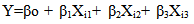 | (1) |
Where:Y = Tumeric yieldXi= TemperatureX2 = Relative humidityX3 = RainfallTable 2. Regression Analysis Result
 |
| |
|
Source: Authors computation using Eviews 7 software.Hence the model becomes: | (2) |
From equation 2, the model shows that when the weather parameters are kept constant the turmeric yield will decrease by -87.80148 (approximately eighty eight thousand kilograms per hectare). The value 0.711734 in the model indicates that the turmeric yield increases approximately by seven hundred and twelve kilograms per hectare when the relative humidity and rainfall are kept constant. The value 0.859925 indicates the yield of turmeric increases when temperature and rainfall are held constant while the value 1.211015 means that the yield of turmeric increased, if temperature and relative humidity are kept constant. Also the R-squared value (0.615968), this means approximately 62% of the variation in the yield of turmeric is explained by the three explanatory variables while 38% remain unexplained. Other test where also carried out like Durbin-Watson statistics (1.647539), Akaike information criterion (7.082215), Prob (F-statistic: 0.011992), Adjusted R-squared, etc.CorrelationIt is pertinent to note that Table 3 is a table of correlation coefficients between each pair of variables in which principle components can be computed. Table 3 confirms that there exists a relationship between the variables.Table 3. Correlation on the average yield and the explanatory variables of turmeric
 |
| |
|
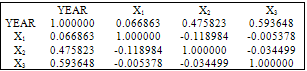
Source: Authors computation using Eviews 7 software.Principal Component Analysis and Orthonormality PlotOrthogonality occurs when two things can vary independently, they are uncorrelated, or they are perpendicular. The essence of this section is to ensure that the explanatory variables are linearly independent also to check multi-colinearity among the variables. Here the correlation table (table 3) is used for the computation of the principal component using Eviews 7. | Figure 1. Orthonormal loading plot |
In figure 1, the orthonormal loading of the explanatory variables are plotted and the results of this plot are as given in Table 4.| Table 4. Result from the orthonormal loadings |
| | Variables | Orthonormal loadings | | Y | 2(0.71,0.05) | | X1 | 5(-0.01,0.66) | | X2 | 8(0.43,-0.61) | | X3 | 11(0.55,0.43) |
|
|
Source: Authors computation using Eviews 7 software.The Table 4 results are centered at (1, 3) with a standard deviation of 3 in the following directions of 1 in the orthogonal direction. The result shows that the result is in accordance with the apriority theorem on PCA which shows that the explanatory variables are linear independent, see http://en.wikipedia.org/wiki/orthonormality.The component 1 and component 2 of the principal components were plotted on the orthonormal loadings. It was discovered that more than 71 percent approximately of the total variations were explained by the first (two) principal components. The 71 percent accounted for is a very good estimate, which leads to the structural co-efficient of the regression model.
5. Summary and Conclusions
5.1. Summary
This paper examines whether total variation in the dependent variable Y could be explained by few explanatory variables(X’s). It starts by analyzing the descriptive statistics of the set of data which showed that the probability of the explanatory variables computed in table 1, are statistically significant at 5% level of significance. The regression result shows that all the co-efficients are highly statistically significant except humidity. However, for the orthonormality of the explanatory variables, correlation analysis was carried out which lead to orthogonality of the variables.Orthogonality occurs when two things can vary independently, they are uncorrelated, or they are perpendicular.Furthermore, the result of the orthogonal analysis was shown using orthonormality loading plot. This plot shows the individual plot of the variables. The result of orthonormality shows that there is no multi-colinearity between the variables. The graphs were used to depict or confirm that trend or pattern of the explanatory variables. The paper therefore concludes that having isolated the Principal Components, the first two accounted for more than 71% of the variation set; this gives better estimate for the response variable in the absence of multi- colinearity.
5.2. Conclusions
The major objective of this study is to compare the efficiency of PCA and regression analyses in predicting the response variable Y using few explanatory variables(X’s).The PCA and regression analyseswere used. The regression result shows that all the co-efficients are highly statistically significant except humidity. The estimate of the correlation matrix was calculated and its Principal Component Analysis (PCA) was carried out to obtain the latent root (Eigen Value) from which the principal components were extracted. It was discovered that more than seventy one percent (71%) of the total variation were explained by the first (two) principal components. In addition, the pattern or trends of the explanatory variables were illustrated using a visual plots. Also, the linearly independent of the explanatory variables were checked by using the orthonormal loadings which shows that there is no multi-colinearity. Even though, the first and second coefficients in regression analysis are statistically significant, the last coefficient is not. But PCA coefficients are statistically significant using few explanatory variables. This study confirms that PCA is preferred to regression analyses in predicting the response variable Y using few explanatory variables(X’s).
Appendix
| Turmeric Yield and Climatic Variables. |
| | Year | Y: Average Yield(ton/ha) | X1: Temperature (oC) | X2: Relative Humidity (%) | X3: Rainfall (mm) | | 1996 | 32.02 | 28.20 | 42.60 | 56.00 | | 1997 | 33.50 | 25.60 | 46.10 | 60.00 | | 1998 | 42.83 | 29.20 | 42.20 | 58.00 | | 1999 | 52.94 | 25.20 | 48.50 | 62.00 | | 2000 | 62.03 | 28.00 | 54.60 | 63.00 | | 2001 | 52.88 | 25.70 | 58.90 | 53.00 | | 2002 | 47.34 | 29.40 | 45.20 | 66.00 | | 2003 | 52.03 | 27.00 | 53.60 | 64.00 | | 2004 | 68.28 | 29.40 | 58.00 | 69.00 | | 2005 | 58.24 | 24.20 | 41.40 | 67.00 | | 2006 | 47.45 | 27.40 | 56.60 | 61.00 | | 2007 | 35.03 | 23.50 | 53.20 | 58.00 | | 2008 | 36.60 | 28.90 | 41.60 | 57.00 | | 2009 | 42.40 | 29.30 | 48.20 | 52.00 | | 2010 | 49.00 | 27.40 | 42.90 | 69.00 |
|
|
Source: National Root Crop Research Institute Umudike data on turmeric yield.
References
| [1] | AxlerS.,Linear algebra done right (2nd ed.), Berlin, New York: |
| [2] | Chan,E.W.C, Lim, Y,Wong, S., Lim,K.,Tan, S.,LiantoF. and Yong, M., 2009,Effects of different drying methods on the antioxidant properties of leaves and tea of ginger species. Food Chemistry113 (1): 166–172.doi:10.1016/j.foodchem. 2008.07.090 |
| [3] | DohrooN.P.,2007, Diseases of turmeric in turmeric the genus curcuma: CRC press pp. 155-167. www.crcnetbase.com/dio/abs/10.1201/9781420006322.ch6 |
| [4] | HotellingH., 1933, Analysis of a complex of statistical variables into principal components. Journal of Educational Psychology, 24, 417-441 |
| [5] | Jagadeeswaran R., MurugappanV. andGovindaswamy M.,2005,Effect of slow release NPK fertilizer sources on the nutrient use efficiency in Turmeric (Curcuma longa L.)World Journal of Agricultural Sciences 1 (1): 65-69 |
| [6] | Jolliffe I.T. (2002) Principal component analysis, Series: Springer Series in Statistics, 2nd ed., Springer, NY, XXIX, 487 p. 28 illus |
| [7] | Miranda, A., Le Borgne, Y. A. andBontempi, G., 2008, New routes from minimal approximation error to principal component, Neural Processing Letters, 27(3), June |
| [8] | On-line turmeric "Curcuma longa information from NPGS/GRIN". www.ars-grin.gov. Retrieved 2008-03-04., accessed on 14 November, 2011 |
| [9] | Orthonormality;On-line http://en.wikipedia.org/wiki/turmeric., accessed on 12 November, 2011 |
| [10] | PCA On-line;http://www.pcp-net.org/encyclopaedia/pca.Html., accessed on 12 November, 2011 |
| [11] | Turmeric;On-line http://en.wikipedia.org/wiki/orthonormality., accessed on 16 November, 2011 |
| [12] | Pearson, K., 1901. On Lines and Planes of Closest Fit to Systems of Points in Space,Philosophical Magazine2(6): 559–572. http://stat.smmu.edu.cn/history /pearson1901.pdf |
| [13] | Wang, Y., Klijn, J.G., Zhang, Y., Sieuwerts, A.M., Look, M.P., Yang, F., Talantov, D., Timmermans, M., Meijer-van Gelder, M.E., Yu, J. et al., 2005, Gene expression profiles to predict distant metastasis of lymph-node-negative primary breast cancer. Lancet 365, 671-679 |
 Abstract
 Reference
 Full-Text PDF
 Full-text HTML