B. Srinivasa Rao1, R. R. L. Kantam2, K. Rosaiah2, M. Sridhar Babu3
1Department of Mathematics, R.V.R & J.C College of Engineering, Guntur, 522 019, A.P, India
2Department of Statistics, Acharya Nagarjuna University, Guntur, 522 010, A.P, India
3Professional Academy for C.A, Hyderabad, 500 038, A.P, India
Correspondence to: B. Srinivasa Rao, Department of Mathematics, R.V.R & J.C College of Engineering, Guntur, 522 019, A.P, India.
| Email: |  |
Copyright © 2012 Scientific & Academic Publishing. All Rights Reserved.
Abstract
The addition of hazard functions of Exponential model and Gamma model with shape 2 is developed. The probability model is considered and an attempt is made to present the distributional properties, estimation of parameters and testing of hypothesis about the proposed model. The findings are described.
Keywords:
LFRD, EGAFRM, Percentiles
Cite this paper: B. Srinivasa Rao, R. R. L. Kantam, K. Rosaiah, M. Sridhar Babu, Exponential-Gamma Additive Failure Rate Model, Journal of Safety Engineering, Vol. 2 No. 2A, 2013, pp. 1-6. doi: 10.5923/s.safety.201311.01.
1. Introduction
In reliability studies, combinations of components forming series, parallel, k out of n systems are quite popular. The survival probabilities of such systems are evaluated either by the system as a whole or through the survival probabilities of the components that define the system. It is well known that in a series system of a finite number of components with independent life time random variables, the system reliability is equal to the product of the component reliabilities. If f(x), F(x), h(x) respectively indicate the failure density, failure probability, failure rate of a component with life time random variable ‘X’, then we know that the reliability is given by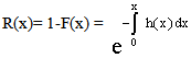 If a series system has two components with independent but non-identical life patterns explained by two distinct random variables say X1, X2, with respective failure densities, failure probabilities, failure rates as f1(x), f2(x); F1(x), F2(x); h1(x), h2(x) then the system reliability is given by
 | (1.1) |
From the above expression we can get the failure density and failure rate of the series system whose reliability is given by (1.1). Such models are already studied in the past with different choices of h1(x) and h2(x). One such situation is the popular linear failure rate distribution [LFRD]. In this model h1(x) is taken as a constant failure rate model, h2(x) is taken as an increasing failure rate (IFR) model with specific choices of exponential for h1(x) and Weibull with shape 2 for h2(x). The failure density, the cumulative distribution function, the reliability and the failure rate of LFRD model are given by | (1.2) |
 | (1.3) |
 | (1.4) |
 | (1.5) |
A hazard rate given in (1.5) is in the form of a straight line equation justifying the name “Linear Failure Rate” for this distribution. A number of researchers made an extensive study on LFRD model. Some recent works in this regard are Bain (1974), Balakrishnan and Malik (1986), Ananda Sen and Bhattacharya (1995), Mohie El-Din et al. (1997), Mahmoud et al. (2006), M.E. Ghitany and Kotz (2007), ABD EL -Baset A. Ahmad (2008), Khedhairi (2008), Sarhan and Zaindin (2009), Sarhan and Kundu (2009), Mahmoud and Al-Nagar (2009), Mazen and Zaindin (2010). Kantam and Priya (2011) have worked out an additive life testing model combining a CFR and DFR model with DFR generated from a Weibull model of shape parameter < 1. The rest of the paper is organized as follows: The distributional properties of our proposed model are given in Section 2. The ML estimations is discussed in Section 3. Discrimination of our model from exponential using likelihood ratio criterion is given in Section 4. Summary and Conclusions are given in Section 5.
2. Distributional Properties
we consider the hazard function of the exponential distribution with parameter ‘λ’ and a gamma distribution with shape parameter 2 and scale parameter v. Then their respective failure rate functions are 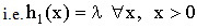 | (2.1) |
 | (2.2) |
The corresponding reliabilities are The series system reliability is
 | (2.3) |
We consider the failure density corresponding to (2.3) as our exponential gamma additive failure rate model (EGAFRM). The probability density function, the CDF, failure rate of EGAFRM are respectively given by | (2.4) |
 | (2.5) |
 | (2.6) |
The mean, median, mode and variance of EGAFRM are | (2.7) |
The median is calculated by taking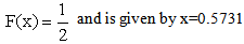 | (2.8) |
 | (2.9) |
The variance is given by | (2.10) |
The central moments and skewness of EGAFRM are given by | (2.11) |
 | (2.12) |
 | (2.13) |
3. Maximum Likelihood Estimation
Let x1, x2 ……..xn is a random sample of size ‘n’ drawn from the EGAFRM with pdf  then the likelihood function is given by
 | (3.1) |
 | (3.2) |
 | (3.3) |
The MLEs of λ,v can be obtained by solving the following likelihood equations 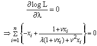 | (3.4) |
and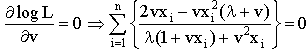 | (3.5) |
The equations (3.4) and (3.5) have to be solved through iteration only with some well known numerical methods and get the MLEs of λ and v say  respectively. However, by using a simple successive method, the ML equations (3.4) and (3.5) can be further simplified and get the following estimators (not ML estimators) for λ,v say
  are obtained
 | (3.6) |
 | (3.7) |
Accordingly the exact variances of the MLEs are not mathematically tractable. However, the asymptotic variance, covariance of the estimates of the parameters are obtained using the following elements of the information matrix: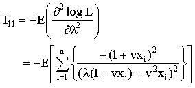 | (3.8) |
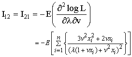 | (3.9) |
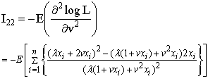 | (3.10) |
The estimated information matrix elements are

 The estimated asymptotic dispersion matrix of the MLEs is given by the inverse of
4. Discrimination between EGAFRM and Exponential Model
We know that the exponential distribution is having a number of preferable properties to be handled for problems of statistical inference. We, therefore are interested in assessing whether exponential distribution is an alternative to our model. In other words given a sample we are interested in studying whether the sample clearly discriminates between our model from that of exponential. Let us designate our distribution EGAFRM as a null population say P0. We call exponential distribution as alternate population say P1. We propose a null hypothesis H0: “ A given sample belongs to the population P0” against an alternative hypothesis H0 : “ the sample belongs to population P1”. Consider a sample from P0. Let L1, L0 respectively stand for the likelihood function of the sample with population P1 and P0. Both L1 and L0 contain the respective parameters of the population. The given sample is used to get the parameters of P1, P0 , so that for the given sample the value of  is now estimated. If H0 is true,
  must be small, therefore for accepting H0 with a given degree of confidence
  is compared with a critical value with the help of the percentiles in the sampling distribution of
  . But the sampling distribution of
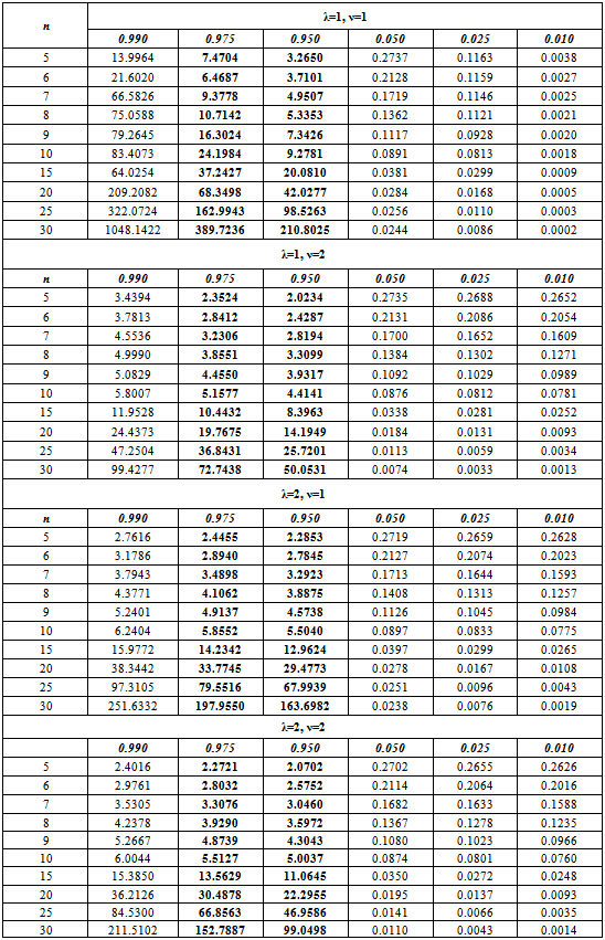
  is not analytical, we therefore resorted to the empirical sampling distribution through simulation. We have generated random samples of size 5(1)10, 15, 20, 25, 30 from the population P0 with various parameter combinations (λ=1,2;ν=1,2) and got the value of L1, L0 along with the estimates of respective parameters for each sample. The percentiles of
  at various probabilities are computed and are given in Table 4.1.In testing of hypothesis we know that the power of a test statistic is the complementary probability of accepting a false hypothesis at a given level of significance. Let us conventionally fix 5% level of significance. So that the percentiles in Table 4.1 under the column 0.05 shall become the critical values. We generate a random sample of sizes 5(1)10,15,20,25, 30 from the population P1 namely exponential. At this sample we find the estimates of the parameters of P1 and P0 using the respective probability models. Accordingly we got the estimates of L1, L0 for the sample from P1.Over repeated simulation runs we got the proportion of values of
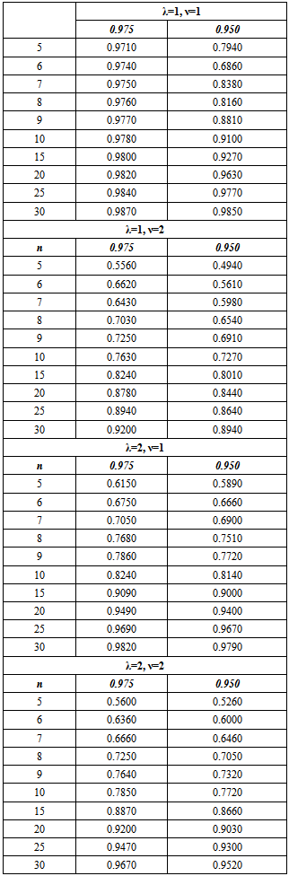
  that fall below the rkespective critical values of Table 4.1. These proportions would give the value of β, the probability of type II error namely β so that the power l- β would be the power. Various power values are given in Table 4.2. We conclude that as long as n is less than 10, a given sample can distinguish between the populations P1 and P0 only with a probability of 10%. Hence exponential can be a reasonable alternative to our model in small samples.
Table 4.1. Percentiles of L1/L0 for various values of λ and v
 |
| |
|
Table 4.2. Power of Likelihood Ratio criterion
 |
| |
|
5. Summary and Conclusions
A combination of Exponential model and Gamma model is developed on lines of the well known linear failure rate model. Estimating equations by ML method are also derived. Its validity as a specified model in the presence of a simpler Exponential model as an alternative is established using a likelihood ratio criterion. In some situations the proposed model stood robust against Exponential.
Acronyms
LFRD- Linear Failure Rate DistributionEGAFRM-Exponential Gamma Additive Failure Rate ModelCFR-Constant Failure RateDFR- Decreasing Failure Rate IFR-Increasing Failure RateMLE-Maximum Likelihood Estimator
References
| [1] | A.AL-Khedhairi. (2008). “ Parameters estimation for a linear exponential distribution based on grouped data”, International, Mathematical Forum, 3 (33), 1643 – 1654. |
| [2] | ABD EL – Baset A. Ahmad. (2008). “ Single and product moments of generalized ordered statistics from linear exponential distributions”, Communications in Statistics – Theory and Methods, 37, 1162 - 1172. |
| [3] | Ammar M. Sarhan and Mazen Zaindin (2009). “ Modified Weibull distribution”, Applied Sciences, 11, 123 – 136. |
| [4] | Ammar M. Sarhan and Debasis Kundu (2009). “ Generalized linear failure rate distribution”, Communications in Statistics – Theory and Methods, 38 (5), 642 – 660. |
| [5] | Ananda Sen and Bhattacharyya, G.K. (1995). “ Inference procedures for the linear failure rate model”, Journal of Statistical Planning and Inference, 46, 59-76. |
| [6] | Bain, L.J. (1974). “ Analysis for the linear failure rate life-testing distribution”, Technometrics, 16 (4), 551 – 559. |
| [7] | Balakrishnan, N. and Malik, H.J. (1986). “Order statiscs from the linear-exponential distribution, part I : Increasing hazard rate case”, Communications in Statistics, Theory and Methods, 15, 179 – 203. |
| [8] | Mahmoud R. Mahmoud – Khalf S. Sulthan – Hassan M. Saleh (2006). “ Progressively censored data from the linear exponential distribution: moments and estimation”, METRON – International Journal of Statistics, LXIV, 2, 199 – 215. |
| [9] | M.A.W. Mahmoud, H.SH. Al-Nagar (2009). “ On generalized order statistics from linear exponential distribution and its characterization”, Stat Papers, 50, 407 – 418. |
| [10] | Mazeen Zaindin. (2010). “ Parameter estimation of the modified Weibull model based on grouped and censored data”, International Journal of Basic and Applied Sciences, 10(2), 122 – 132. |
| [11] | M.E. Ghitany and Samual Kotz. (2007). “ Reliability properties of extended linear failure rate distributions”, Probability in the Engineering and Informational Sciences, 21, 441 – 450. |
| [12] | M.M. Mohie El-Din, M.A.W. Mahmoud, S.E. Abu-Youseff, K.S. Sultan (1997). “ Ordered statistics from the doubly truncated linear exponential distribution and its characterization”, Communications in Statistics – Simulation and Computation, 26 (1), 281 – 290. |
| [13] | R.R.L. Kantam and M.Ch. Priya (2011). “An additive life testing model”, contributed Paper : conference on statistical Techniques in Life-Testing, Reliability, Sampling theory and Quality Control, Banaras Hindu University, Varanasi, Jan 4 -7, 2011. |
 Abstract
 Reference
 Full-Text PDF
 Full-text HTML