1. Introduction

The development and assessment of concentration photovoltaics (CPV) technology is facilitated by the use of optical characterization techniques that qualify the properties of the concentrator in terms of overall optical efficiency; this figure of merit is measured in conditions of perfect alignment with respect to the solar disk, as well as in function of the extent of misalignment [1-5].

The concentration system is usually assemblies of many optical and mechanical parts, so it is useful to proceed to the characterization of the individual components of the system to help their performance analysis. This process can be carried out both experimentally, in laboratory, or virtually, by using optical software. In this last case, the single components are assembled in a CAD model and tested in optical simulation software to extract the performance expected for the system as a whole.

In this paper we will discuss two methods of characterization of concentration units, one of them having proved to be extremely powerful to measure the efficiency losses due to misalignment of the concentrator from the solar disk [6-24]. The characterization methods will be applied to two small concentration units called "Rondine" developed by the company CPower Srl [25-30].

Before explaining the two methods of characterization, it is useful to briefly summarize the basic concepts that underlie the behaviour of a solar concentrator [31-39].

A solar concentrator is an optical device that works mainly on direct solar radiation, and, in its simplest form, can be realized by using lenses or mirrors. In the first case we refer to refractive concentrators, in the latter case to reflective concentrators. In reality, a concentrator can be more complex, designed combining more elements of refractive and reflective nature. In a 3D or point-focus solar concentrator the incident rays are forced to cross increasingly smaller areas and at the same time to increase their angular divergence θ, as established by Liouville's theorem: A · sin²θ = const (valid for an ideal concentrator without optical losses). So, the concentrator increases the incident flux density, starting from about 900 W/m² (a value typical of clear sky conditions) up to values, which depend on the optical concentration ratio, :

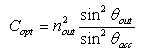(1)

where is the maximum angular divergence of output rays, is the acceptance angle, that is the angle at which the efficiency of the concentrator drops to the 50% of the maximum, and is the index of refraction of the medium embedding the receiver. When the SC is irradiated by the direct component of the sun, to collect all the direct irradiation it is necessary to have , where is the maximum divergence of direct sunlight incident on the Earth's surface, determined by the particular geometry of the Sun-Earth system [40]. The maximum optical concentration ratio is reached when the divergence of rays at output is = 90° and :

(2)

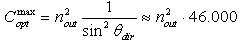
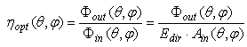
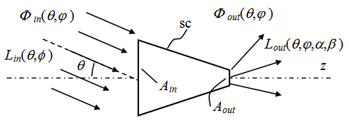
Eq. (2) establishes the thermodynamic limit of the concentration ratio for a concentrator operating on the Earth surface. The process of optical concentration does not generally occur with unitary efficiency, as part of the flux is rejected back due to the particular geometry of the concentrator or absorbed by the constituting materials. The optical efficiency is defined as the ratio of the output to the input flux and significantly depends on the orientation of the concentrator with respect to the solar rays (see fig. 1). 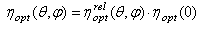Besides the absolute efficiency , it is useful to consider the relative, or normalized, optical efficiency 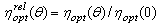, which contains only the information of the effect, on the light collection efficiency, of misalignment of concentrator with respect to the solar disk.

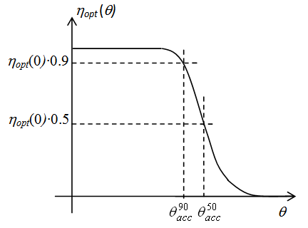Figure 1. The overall optical properties of a solar concentrator are summarized by the transmission efficiency curve . Here it is shown the typical efficiency curve of a solar concentrator based on the nonimaging optics (NIO). The efficiency curve contains the relevant information of the acceptance angle, the angle at which the efficiency drops to the 50% of the maximum value (to the 90% of the maximum value for PV applications)

Conventional solar concentrators such as basic parabolic mirrors or Fresnel lenses are very sensitive to Sun disk misalignment, but the advent of NIO ("nonimaging optics” or “optics without image") by Winston [31-34, 36, 37] has revolutionized this research sector, enabling to realize concentrators based on new concepts; hereafter we mention the concept of "edge ray principle".

Classic NIO concentrators, also known as "light cones", are the CPC (Compound Parabolic Concentrators); their geometry is particularly suited to achieve high concentration ratios, near to the thermodynamic limit of Eq. (2). In addition, the NIO concentrators have the property of being less sensitive to the incidence angle of light up to the acceptance angle (see Fig. 1), compared to imaging optics designs.

2. The “Rondine” PV Concentrator

The “Rondine” PV concentrator is a modular structure composed of original nonimaging optical units of the class of light cones, derived from the compound parabolic concentrator (see Figs. 2-4) [25-30]. The concentrator length has been defined to obtain about only one reflection for the rays entering parallel to the optical axis of the concentrator and striking the surface, to reduce the optical losses due to multiple reflections. The elementary concentrator has a squared input window and lateral apertures; in this way, many elementary units can be closely joined in a dense array, without losses due to the packaging. This approach gives the same angular tolerance like having perfectly flat-mirrored surfaces placed on the cut lateral planes. The absence of a symmetrical rotational axis gives an irradiance distribution on the solar cells without one single hot spot; this illumination profile reduces possible losses in FF due to the distributed series resistance of the devices.

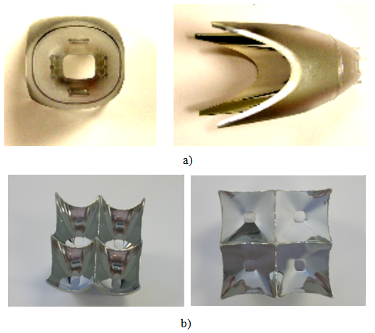Figure 2. a) Rondine Gen1 single optical units based on NIO (Non Imaging Optics); it is visible the exit aperture with its quasi-rectangular shape. b) Rondine Gen2 single optical units; it is visible the exit aperture with its quasi-squared shape

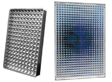Figure 3. CPV modules “Rondine” realized by Rondine Gen1 (left) and Rondine Gen2 (right) single optical units. Rondine Gen1 CPV data: Wp = 95.5 W; Eff = 12.3%; C = 25X. Rondine Gen2 CPV data: Wp = 120 W; Eff = 16%; C = 20X

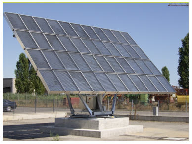Figure 4. First installation of a 4kWp tracking Rondine Gen1system, at Ostellato (Ferrara, Italy)

Until now, two different designs of optical units were manufactured: first generation Rondine Gen1 and second generation Rondine Gen2. They differ in dimension and shape: Rondine Gen1 has a square input aperture of 70-mm side and a quasi-rectangular exit aperture of 17.6 mm x 13.3 mm (see Fig. 2a), whereas Rondine Gen2 has a square input aperture of 35-mm side and a quasi-squared exit aperture of 8-mm side (see Fig. 2b).

The optical properties of the reflective surface of this concentrator can be approximated, at a wavelength of 0.5μm, as: specular reflectance R = 0.85, absorbance A = 0.09, integrated BRDF = 0.06.

An estimate of the relative power efficiency of a Rondine Gen1 CPV module versus the misalignment angle of pointing resulted in an angular acceptance of about 6.0° along one module axis and about 3.0° along the other one. The discrepancy found between the optical angular acceptance of the single concentrating units and that of a complete module, which was about 1.5-2.0°, has to be attributed to a non-perfect coupling between concentrating units and solar cell, and to errors in the manual assembling of the different parts of the modules.

3. “Direct” Characterization Method

With “direct” characterization method we briefly intend the “Direct Collimated Method”, DCM, whose detailed theoretical treatment can be found in refs [6, 7]. Here we summarize the basic principles of this method. The DCM consists, in principle, in drawing the optical transmission efficiency curve of the concentrator when it is irradiated by a parallel and uniform beam at different orientations in space, the transmission efficiency being defined as the ratio between output and input flux as function of the polar θ and azimuthal φ angles of incidence of the beam:

(3a)

where is the area of input aperture projected along direction (θ, φ). If the input aperture is planar and with area A_in , Eq. (3a) simplifies as:

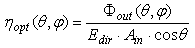(3b)

Eq. (3) implies the use of a parallel beam, but this can be realized only by using optical simulation programs, not in practice [6]. We have to distinguish therefore, just by now, that Eq.s (3a), (3b) will be applied with a parallel beam in optical simulations, and with a quasi-parallel beam in experimental measurements. As a solar concentrator works prevalently with the direct solar beam, of ±0.27° angular divergence, we conclude that the most appropriate beam to use for the experimental measurements is a ±0.27° divergent quasi-parallel beam. This specification has some consequences for the purposes of comparing the two methods proposed here, that is the “direct” and the “inverse” one, both when they are applied as simulations that when applied experimentally; These consequences will be discussed from time to time when they will need.

The basic scheme of DCM is shown in Fig. 5. L_dir (θ, φ) (W/m²·sr) is the average radiance from (θ, φ) direction.

Figure 5. Basic scheme of the Direct Collimated Method (DCM)

The optical efficiency of Eq. (3) can be expressed as:

(4)

Where is the efficiency relative to 0° incidence. To draw out the optical efficiency curve experimentally, we have to prepare the ±0.27° divergent beam with a uniform irradiance distribution on the cross section and with an orthogonal section area sufficiently large to include the input aperture area of the concentrator. Then it is necessary to measure the flux Φ_out (θ, φ) collected at the exit aperture of the concentrator for different orientations of the concentrator respect to the incident beam.

The polar incident angle θ is sufficient to define the orientation of the concentrator when it has a cylindrical symmetry, like a standard CPC; for other concentrators, like the “Rondine” in this paper, it is necessary to consider also the azimuthal incident angle φ. We will limit, however, our study with the DCM method only to two azimuthal orientations for the Rondine Gen1, those parallel to the two edges of the input aperture profile, and to one azimuthal orientation for the Rondine Gen2, that parallel to one edge of input aperture profile.

To prepare the collimated beam we use a light source (ls) which illuminates two coupled integrating spheres (is₁) and (is₂) (see the two configurations of Fig. 6 that will be discussed later): the light produced at the output window (w) of (is₂) is a diffused light with Lambertian intensity distribution. The use of two integrated spheres instead of one is preferred to have a better integration of light inside the sphere used as source of diffused light. If the window (w) is placed at the focal point of the parabolic mirror (pm₁), then the light beam reflected by the mirror is quasi-collimated with a maximum angular divergence fixed by the window dimension and the mirror focal length. To obtain the 0.27° divergence, it is necessary to adjust the ratio between window (w) diameter and mirror focal length to ~1:100, the same ratio between Sun diameter and Sun-Earth distance. The quasi-collimated beam is then selected by diaphragm (di) and directed to the solar concentrator (sc), whose output flux is measured by coupling the exit aperture with a third integrating sphere (is₃), and measuring the irradiation level inside the sphere by a suitable radiometric unit. By this way the optical efficiency of the concentrator relative to the on-axis direction (0° incident angle) is obtained.

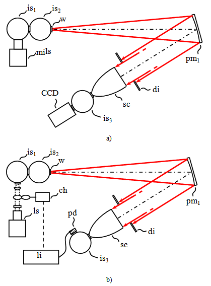Figure 6. Schematic principle of the direct method used for the measure of the output flux. a) Configuration A: the source (ls) is a continuous light and the radiometer is a CCD. b) Configuration B: the source (ls) is a chopped light and the radiometer is a lock-in amplifier. The diameter of window (w) is 5 mm and the focal length of (pm1) is 500 mm

To get the absolute optical efficiency, , it is necessary to make a further measurement of . This is done by removing the concentrator (sc), decoupling it from sphere (is₃), and orienting the collimated beam from mirror (pm₁) towards a second parabolic mirror (pm₂) (see Fig. 7), which will provide to re-focalise the beam inside the same integrating sphere (is₃). For this measurement, it is required the knowledge of the spectral reflectance of (pm₂).

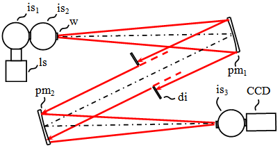Figure 7. Schematic of the experimental configuration A applied to the measure of the flux at 0° incidence. A similar schematic applies for the experimental configuration B

In this paper, the apparatus used for the application of DCM has been realized, whenever possible, by using low-cost components. The three integrating spheres, of different diameter, where realized in laboratory starting from commercial plastic globes, which were worked with an original multi-step coating process in order to have an opaque, highly reflective and diffusive internal wall [24] (see Fig. 8). In this way we were able to reach the standards commonly requested to a good commercial integrating sphere realized using an Aluminium substrate [41], but with a cost reduction of about hundred times.

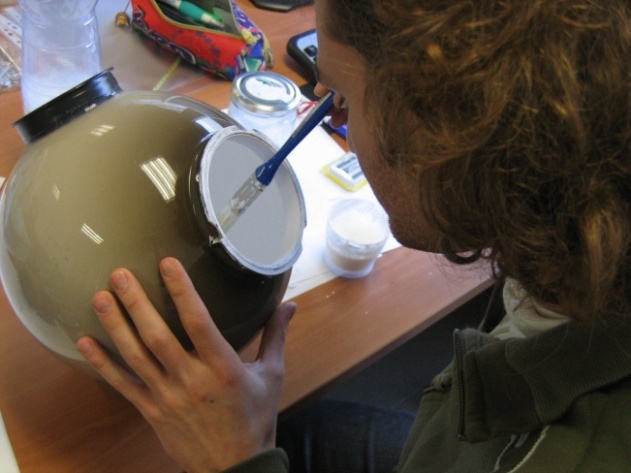Figure 8. A plastic globe is undergoing manufacture for the coating of the inner layer of BaSO4

Here we have to distinguish between two different experimental configurations, one the evolution of the other, and both used for the measure of transmission efficiency (see Fig. 6). In the first one, called configuration A, we have used a continuous light; in the second one, called configuration B, we have used a pulsed light. In both configurations the light source was a commercial fluorescent lamp (ls) (Philips 23W, CDL865), with a spectrum near to that of the Sun (T=5500-6000K), facing the inside of the integrating sphere (is₁), that in turn was cooled by a fan to avoid the overheating of the plastic globe. In the configuration A, as detector for flux measurements, we have used an Hamamatsu 1394 C8484-05G CCD camera, facing the inside of the integrating sphere (is₃), operating like a normal photodetector; the flux being measured by averaging the intensity of the digital CCD image.

The CCD, due to its high sensitivity, is the only means of measuring the continuous, very low flux transmitted by the Rondine to the integrating sphere (is₃). The parabolic mirror (pm₁) was a low cost, commercial mirror with a focal length of 50 cm. Fig. 9 shows a photo of the experimental set-up used with configuration A. The intensity distribution (irradiance) of light on the cross section of the collimated beam is shown in Fig. 10. It was obtained by projecting the parallel beam on a lambertian diffuser and measuring the intensity distribution by means of the CCD. The intensity profile shows a flatness modulation of around ±8%, due to the low quality of the parabolic mirror. This, as we will see, will produce a small distortion of the efficiency curve and a small alteration of the acceptance angles.

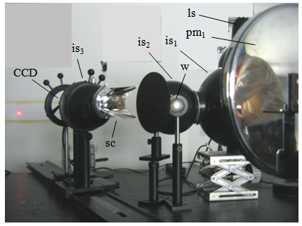Figure 9. Photo of the apparatus for DCM measurements with configuration A

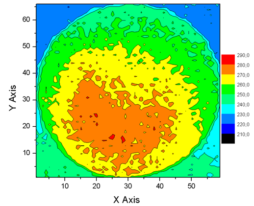Figure 10. Intensity distribution of light on the cross section of the quasi-collimated beam produced for DCM in the configuration A

In the configuration B, the same fluorescent lamp was mounted at the centre of the integrating sphere (is₁), which was cooled again by a fan (see Fig. 11a). The lambertian light from window (w) (15 mm diameter) of (is₂) was modulated by the chopper (ch) and directed towards the mirror (pm₁) (see the box in Fig. 11a and Fig. 11b). Here the mirror is a high quality, high cost, Pyrex parabolic mirror, of 300mm diameter, 50mm thickness, F/5 (1500 mm focal length), λ/ 8 quality [42]. In the configuration B, the flux measurements at the exit aperture of Rondine were carried out in two modes.

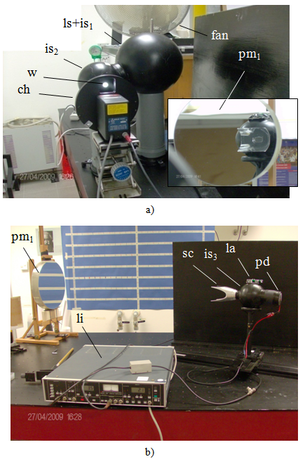Figure 11. Photos of the apparatus for “direct” measurements with the configuration B. a) Light source section. The small box shows the high quality parabolic mirror. b) Receiver section. The “Rondine” has bounded on the top a diode laser (la) used for the alignment with the mirror

In the first one, the SPHERE mode, we have coupled the exit aperture of Rondine to the (is₃) integrating sphere, provided with an internal photodiode (pd) (an high efficiency solar cell of 4 cm² area), as illustrated in Figs. 6b and 12a; in the second one, the CELL mode, we have closed the Rondine exit aperture with an high efficiency solar cell (dimensions of active area: 16mm x 12mm), the same used in the CPV module (see Fig. 12b).

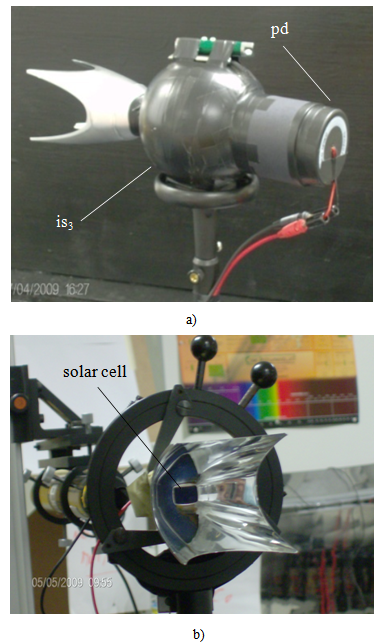Figure 12. a) Photo of the Rondine Gen1 closed on the integrating sphere (is3) (SPHERE mode); b) Photo of the Rondine Gen1closed on the high efficiency solar cell (CELL mode)

In both cases, the photodiode and the solar cell were connected to the lock-in amplifier (li) Kandel Electronics 5210 operating at 600 Hz (see Fig. 11b). The reason why we adopted two different receivers for measuring the flux transmitted by the Rondine is the following: in the case of SPHERE, the integrating sphere behaves as an ideal receiver, or nearly so, then the measure gives the transmission efficiency of Rondine itself, as a simple optical concentrator, regardless of the type of receiver used; in the case of CELL, on the other hand, the measure gives the transmission efficiency of the system Rondine + PV receiver, and then the more realistic angle-resolved optical performance of the Rondine PV concentrator when mounted on the CPV module.

The projection of the quasi-parallel beam on a lambertian diffuser is shown in Fig. 13. The intensity distribution map is shown in Fig. 14. The map shows flatness better than 0.5% within 100 mm width; it was greatly improved after the use of the new parabolic mirror [42].

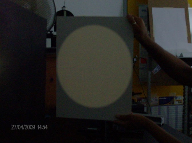Figure 13. Projection of the parallel beam on a lambertian diffuser after reflection from pm1

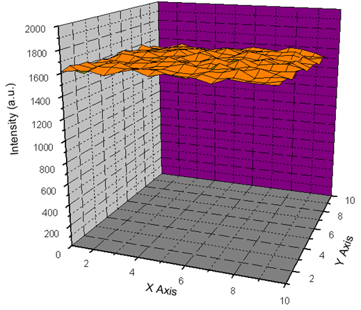Figure 14. Plot of the intensity of light measured on a 100x100mm2 square cross section of the parallel beam after reflection from pm1

4. “Inverse” Characterization Method

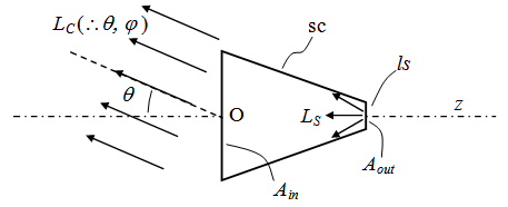
The “inverse” method, initially known as ILLUME (Inverse Illumination Method), was later revisited and improved, assigning the new name of “Inverse Lambertian Method” (ILM). The theoretical details are given in ref. [6].

The ILM greatly simplifies the experimental apparatus for measuring the angle-resolved transmission efficiency, both relative and absolute, and drastically reduces the number of measurements. The method consists in irradiating the concentrator (sc) in a reverse way by placing a planar Lambertian light source (ls) of uniform radiance L_S at the exit aperture, and in measuring the radiance L_inv(θ, φ) of the light emitted by the concentrator from the input aperture as function of the different orientation in space, characterized by the polar emission angle θ and the azimuthal emission angle φ (see Fig. 15) (here we use for simplicity the same symbols for the angular direction of the rays incoming to and out coming from the input aperture). When inversely illuminated, the concentrator becomes a light source whose radiance will no longer be constant, because the concentrator changes the angular distribution of the rays emitted by the lambertian source (ls), before they are emitted from the entrance opening.

Figure 15. Basic scheme of the inverse lambertian method (ILM)

Differently from the DCM, where measurement of Φ_out(θ, φ) every time requires changing the orientation of the concentrator with respect to the quasi-parallel beam, the measure of L_inv(θ, φ)is now immediate, because it is obtained from the fast processing of a single image produced on a planar screen (ps) by the inverse light (see Fig. 16). The processing procedure depends however on the type of measurement. If the inverse method is simulated at a computer, the planar screen (ps) is assumed as an ideal absorber, and the irradiance E(θ, φ) of the incident light is directly measured. If the inverse method is applied experimentally, on the contrary, the planar screen must be a white diffuser with lambertian properties and a CCD is used to record the inverse light there projected. In this case, the irradiance of incident light is measured indirectly, deriving it from the intensity of the CCD image I_CCD(θ, φ).

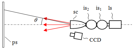Figure 16. Schematic of the experimental ILM apparatus

The only foresight to follow when applying the inverse method is that the planar screen, oriented perpendicular to the optical axis of the concentrator and illuminated by the inverse light, must be placed at a distance d from the concentrator much higher than the linear dimensions of the input aperture, in order to have an adequate angular resolution for the profile of optical efficiency. For example, for a circular input aperture of diameter D, the angular resolution (uncertainty) Δθ_res for all the points (in a circle) of the screen characterized by the polar emission angle θ are given by:

(5)

The angular resolution is the worst on the optical axis:

(6)

and improves at increasing θ. Since the angular range of light emission is generally small, we can assign to the points of the emission radiance the angular resolution obtained by Eq. (6). The need to have d >> D implies some limits to the application of the ILM in laboratory, where distance d can be of the order of some meters. For example, a concentrator of 10-cm aperture size requires a screen at 5 m to have a resolution of at least ~0.5° on the optical axis. This is the only drawback of the ILM when applied experimentally. When ILM is simulated on the computer, on the other hand, it is easy to set a sufficiently high value of d /D to obtain the desired resolution, of course by using a ray-tracing with many rays and then with greater processing time. The choice of d, then of the angular resolution, must be made mainly taking into account the expected value for the angle of acceptance. A resolution of ~0.5°, for example, cannot be tolerated for an acceptance angle (at 50%) of about 1° or less, while it is acceptable for an acceptance angle of at least 5°, as is the case of the Rondine concentrators.

Referring to the measurement of , it may happen that the optics of the CCD is not always adequate to capture the entire inverse image at the distance d between concentrator and screen. In this case, that we have effectively experienced, it is possible to double the optical path between the screen and the CCD interposing a mirror (mi) between the CCD and the screen, as shown in Fig. 17.

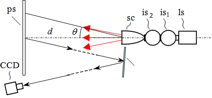Figure 17. When the full inverse image on the screen cannot be captured by the CCD objective, then the help of a mirror (mi) can double the optical path between screen and CCD

With simulation measurements, the irradiance on the planar screen is transformed into the radiance L_inv(θ, φ) of the concentrator by the following expression (see the Appendix):

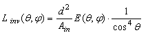(7)

where A_in is the input aperture area and d is the on-axis distance between the planar screen and the centre O of the input aperture of the concentrator. To obtain the relative profile of the inverse radiance, , that is the radiance normalized to the 0° value, it is sufficient to measure the normalized irradiance on the screen, :

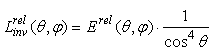(8)

The factor (cosθ)^-4 takes into account the fact that the screen is a flat surface rather than spherical, and the points on the screen (ps) are not located at the same distance from the centre of the opening entrance, which is the point from which we measure the angles.

When the inverse method is applied experimentally, Eq. (7) modifies and becomes (see the Appendix):

where f is the focal length of CCD and R the reflectivity of the lambertian screen. The normalized radiance now becomes:

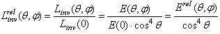
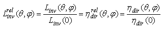
We have demonstrated [6, 8-11, 13, 15, 18] that the relative inverse radiance profile coincides with the relative optical efficiency profile of the concentrator operating in the direct mode (DCM) when the direct beam is strictly parallel. When the direct beam is not strictly parallel, we have to take account of its divergence and to put it as the uncertainty on the measured efficiency. We have therefore for the optical efficiency of the concentrator:

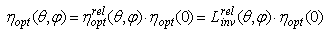(9)

where is obtained from Eq. (8) or (8’) depending if we are operating with a simulation program or with experimental measurements. We conclude this part highlighting the fact that the radiance summarizes all information relating to the light collection properties of the concentrator in relation to its orientation with respect to the solar disk.

The inverse method as discussed until now seems to allow determining only the relative angle-resolved optical efficiency of the concentrator, by processing the intensity image produced on the planar screen by the concentrator irradiated in the inverse way. To obtain the absolute efficiency as indicated by Eq. (9), we should ask the direct method for help to measure the on-axis optical efficiency . If it were really so, we should need to set-up also the direct method apparatus just for one measurement, and the advantages of the inverse method in terms of simplicity of the experimental apparatus should be lost. Fortunately, new developments of the theory [6, 9, 10] provide a way of obtaining also by the inverse method. 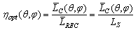It can be shown in fact that the on-axis efficiency can be obtained by the expression:

(10)

where and are radiances measured on the image recorded by the CCD camera oriented towards the input aperture of the concentrator irradiated in the inverse mode (ILM) (see the schematic of the apparatus in Fig. 18). is the average radiance of the whole input aperture, whereas is the radiance of the receiver, the exit aperture, corresponding to the radiance of the Lambertian source.

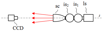Figure 18. Experimental set-up for determining the on-axis optical efficiency of the concentrator. The CCD camera is turned towards the concentrator irradiated in inverse mode and the image of the input aperture is recorded

It should be emphasized that Eq. (10) is easily applied to concentrators for which the exit aperture is visible from the input aperture, like a CPC or any other concentrator realized only by reflective optics. For concentrators with refractive components in the front, the measure of becomes independent of that of and requires the removal of those components. As the optical efficiency ≤ 1, we will always have ≤ .

To produce the Lambertian source on the back of the concentrator (sc), we can use a light source (ls) and a pair of integrating spheres (is₁) and (is₂) as already done when applying the direct method (see Fig. 19a). A Xenon arc lamp is the best choice to simulate the direct solar spectrum, whereas the integrating sphere is the best choice to obtain a lambertian light source [43-47]. The concentrator is grafted on to the output window of (is₂) as shown in Fig. 19b, where it is also shown the “baffle” (ba) at the centre of the sphere. The baffle has the function to filter the direct light coming from sphere (is₁) and assures a lambertian distribution of light at the exit window of (is₂). The planar screen is placed in laboratory at a proper distance from the source and there the characteristic light image, leaved by the inverse beam as a fingerprint, is produced (see Fig. 19c).

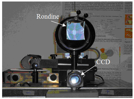
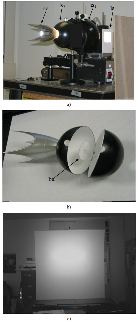Figure 19. a) Photo of the ILM (ex ILLUME) apparatus during characterization of the Rondine Gen1. b) Photo of the Rondine Gen1 "grafted "on the integrating sphere (is2). c) The planar screen and the ILM image produced on it

The inverse image produced on the screen is then analysed by means of the HiPic software operating with the Hamamatsu CCD camera. Fig. 20 shows, as an example, the intensity profiles recorded along the horizontal (x-axis) and vertical directions (y-axis) of the image produced by the Rondine Gen1 concentrator.

Figure 20. Analysis by HiPic of the ILM image produced by the Rondine Gen1. The irradiance profiles, traced along the horizontal (x-axis) (a) and the vertical (y-axis) (b) directions, need to calibrate the polar angle of the points along the corresponding axis

Some black dots are placed at fixed distances on the screen (ps) and used as reference points of a Cartesian frame for measuring the distances on the screen and then obtaining the polar and azimuthal angles associated to any point on it.

During the calibration of distances, the horizontal and vertical profiles were traced in such a way to take in the dots, which appear in the profiles as thin peaks (see Fig. 20).

To get the correct irradiance profile on the screen, it could be needed to adjust the intensity and shape of the image for possible effects of perspective; this depends on the actual position of the CCD camera respect to the optical axis and is not necessary when the camera is placed very close to concentrator (see Fig. 21). If necessary, the perspective correction can be applied by using a program developed by us [48, 49]. Once known the distances between the dots, the calculation of angles is straightforward.

The photo of the front side of the Rondine Gen1 irradiated in the inverse mode is shown in Fig. 21. The CCD camera is placed very close to the concentrator and on the plane of its input aperture.

Figure 21. Photo of the Rondine during ILM measurements. The CCD is placed just below at short distance

Fig. 22 shows the detail of the entrance aperture sight in front, outlined by the red frame, with the central region REC (blue frame) corresponding to the Lambertian source. The central region is the most lit of the image, because it is the direct source of inverse light, which does not undergo attenuation inside the concentrator. If the lambertian source is made well, moreover, the image of REC is very uniform, as it represents the constant radiance of an integrating sphere. Following Eq. (10), the on-axis efficiency is equal to the ratio between the average intensity of the red region and the uniform intensity of the blue region.

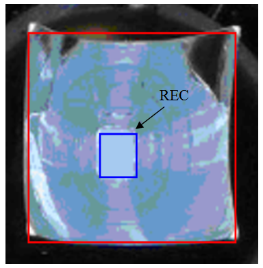Figure 22. Image of the front side (on-axis) input aperture of Rondine1. The blue frame surrounds the area of the receiver (REC); the red frame surrounds the total input area

Indeed, if we would take this measure at different CCD orientations, we would precisely get, the absolute transmission efficiency:

(11)

By doing so, however, we would fall back into the same drawbacks of direct method, because we would need again to carry out a measure for each orientation of the CCD, so we will not use this method to get . Eq. (11) applies at any distance between the CCD and the concentrator, since the radiance is constant with distance.

5. Experimental and Simulated Results

5.1. Transmission Efficiency by the Direct Method

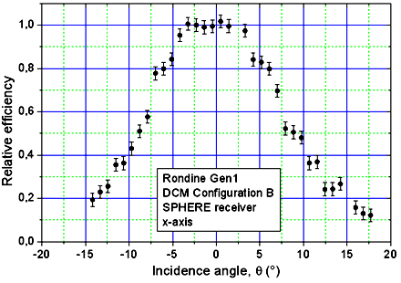
We start discussing the results of measurements made by the DCM, configuration A. Fig. 23 shows the experimental curves of optical efficiency obtained for the Rondine Gen1 concentrator. The dashed rectangle represents the exit aperture of the concentrator and the arrow indicates the direction of the plane of incidence of the quasi-parallel beam. The exit aperture of the concentrator however is not a simple rectangle as the corners are smoothed (see Fig. 2a). The x-profile (y-profile) has been traced parallel to the major (minor) edge of the exit aperture. Fig. 23 shows that the x-profile and y-profile are slightly distorted, as expected as an effect of lack of symmetry of the intensity distribution of the parallel beam (see Fig. 10). The acceptance angles measured for the x-profile and y-profile at 90% of the 0° efficiency are 4.4±0.2° and 6.5±0.2°, respectively. The acceptance angles measured for the x-profile and y-profile at 50% of the 0° efficiency are 9.2±0.2° and 9.6±0.2°, respectively. As it can be seen from Fig. 23b, the y-axis efficiency at 0° does not correspond to the maximum value, due to the slight distortion of the profile. The errors assigned to the acceptance angles are random errors derived from the intensity measurements carried out by the CCD camera inside the integrating sphere (is3), so they do not include systematic errors like those introduced by the use of a non perfectly symmetric and uniform beam (see Fig. 10), nor the angular divergence imposed to the beam.

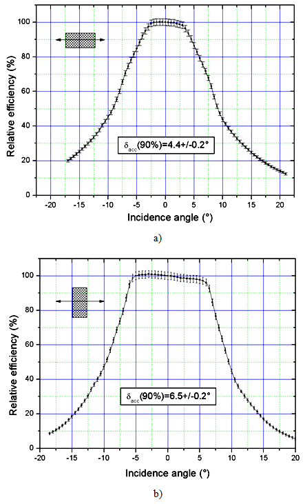Figure 23. a) Relative efficiency of the Rondine Gen1 concentrator traced along the x-axis. b) Relative efficiency of the Rondine Gen1 concentrator traced along the y-axis

The tracing of the efficiency curve has required in both cases 77 measurements with 0.5° steps. In total we have made 154 measurements for obtaining the optical efficiency profile along only two azimuthal directions in space, in practice one day of work.

As we shall see soon after showing the results of the inverse method, it is sufficient a single measurement, that is the recording of a single image, to obtain the efficiency profile along any azimuthal direction of the incident parallel beam.

We continue discussing the results of measurements made by the DCM, configuration B. By using a SPHERE type receiver, we expect to obtain for the Rondine Gen 1 similar results to those obtained with the configuration A, or even better, considering the use of a high-quality parabolic mirror, then of a more uniform quasi-parallel direct beam. Instead, as we shall see, the results will be more critical because of the very low level of the signal to the lock-in input.

Fig. 24 shows the experimental curve of optical efficiency along the x-axis of the Rondine Gen1 concentrator. The curve of Fig. 24 is similar to that of Fig. 23a, but is affected by higher random errors. The acceptance angles measured for the x-profile are 4.2±0.4° at 90% of the 0° efficiency and 8.9±0.4° at 50% of 0° efficiency; the errors have doubled compared to the configuration A. These data, however, are compatible with those measured with the configuration A (see Fig. 23a).

Figure 24. Normalized efficiency of Rondine Gen1 traced along the x-axis with the DCM, configuration B, and SPHERE type receiver

The following results regard the measurements on Rondine Gen1 of DCM, configuration B, and CELL receiver. The curve of transmission efficiency measured along the x-axis and y-axis are shown together in Fig. 25.

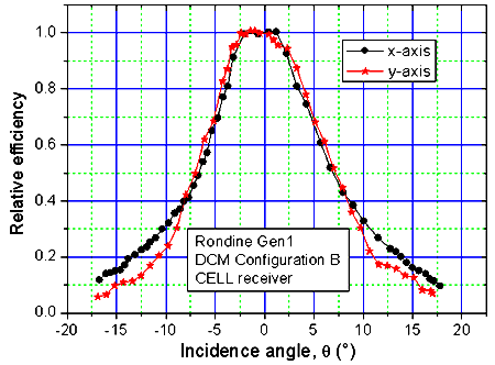Figure 25. Relative efficiency of Rondine Gen1 traced along the x-axis and y-axis with the DCM, configuration B, and CELL receiver

As regards the x-axis profile, we observe that there is a narrowing of the curve compared to measurements with the SPHERE receiver. The acceptance angles are in fact: 2.8±0.2° at 90% of 0° efficiency (≈35% narrowing) and 6.8±0.2° at 50% of 0° efficiency (≈25% narrowing).

As regards the y-axis profile, we observe an ever stronger narrowing of the curve respect to measurements with the SPHERE receiver (configuration A). The acceptance angles are in fact: 3.3±0.2° at 90% of 0° efficiency (≈50% narrowing) and 7.2±0.5° at 50% of 0° efficiency (≈25% narrowing). From Fig. 22 we note that the use of a solar cell as receiver has determined, besides the narrowing of the efficiency curves, also their equalization.

The modification of the transmission efficiency at changing the receiver from SPHERE to CELL mode could be explained by different angle-resolved absorption properties of the solar cell respect to an ideal absorber like the integrating sphere. To investigate this fact, we need to study two aspects of the problem: i) to measure experimentally the absorption of the cell as function of the polar incidence angle of a parallel beam to check how much its relative response deviates from that of an ideal absorber; ii) to measure, by simulation, the distribution of the angle of incidence of light on the solar cell as function of the incidence of light at input of the Rondine concentrator. The two results should then put together to see if the behaviour of the Rondine+cell, summarized by Fig. 25, is justified.

From now on we will indicate with symbols α and βrespectively the polar and azimuthal angles of incident rays on the exit opening of Rondine, and then also on the solar cell.

To measure the angle-resolved absorption of the solar cell, we have arranged an experimental set-up like that shown in Fig. 26. After removing the Rondine from the receiver station, the bare cell was fixed on a rotating table provided with a goniometer, short circuited on a 1 Ω resistive load and connected to the lock-in. Before the measurements, the cell was aligned with the parallel beam reflected by the parabolic mirror to check the 0° orientation. We finally measured the short circuit current as function of polar angle αof the parallel beam. Fig. 27 shows the angle-resolved short circuit current normalized to 0° incidence, compared to the cosine function.

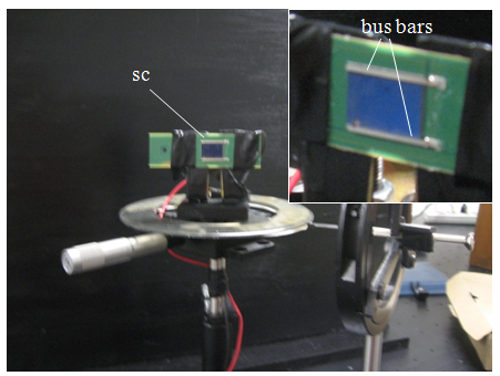Figure 26. Characterization of the solar cell under a quasi-parallel beam incident at different polar angles. The cell is placed on a rotating base provided with a goniometer. The box shows the bus bars of the cell

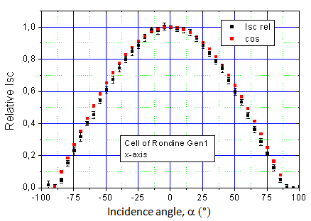Figure 27. Plot of the short-circuit current Isc of the Rondine Gen1 cell, normalized to 0° incidence, as function of the polar incidence angle α. The Isc is compared to the cosine function

The response of the cell is similar to that of an ideal absorber, so we think it is not responsible of the narrowing of the transmission efficiency curves, as deduced from Fig. 22. The relative deviation of the normalized short-circuit current of Fig. 27 from the cosine function was calculated and shown in Fig. 28 as relative loss function, Λ(α):

(12)

where angle α is expressed in degrees.

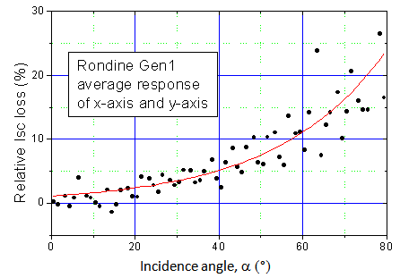Figure 28. Relative percent loss of the short circuit current normalized function with respect to the cosine function, calculated from the measurements on the Rondine Gen1 solar cell by the experimental configuration of Fig. 26. The data are the average response of the cell at light with the incidence plane aligned to the x-axis (β=0°) and to the y-axis (β =90°)

The data refer to both x-axis (β= 0°) and y-axis (β = 90°) azimuthal orientations.

We now proceed, as established, with the second step, investigating the angular distribution of light transmitted by the exit aperture of Rondine (see Section 5.6 for details of this simulation). To this purpose, we have used a commercial optical code, by which we have performed all the ray-tracing simulations necessary to reproduce the DCM method (and the ILM method, as we will see in the next section). Before beginning the simulations, however, we needed to modify the entrance opening of the Rondine. The current shape of the Rondine, in fact, does not allow to properly set-up a parallel beam at input because its entrance aperture has a non-planar profile (see Eq.s (3a) and (3b)).

To remedy this, it was necessary to box laterally the frontal section of Rondine adding four walls as ideal mirrors, in such a way to have a simple squared entrance aperture (see fig. 29). The addition of the four front mirror walls does not alter significantly the optical behaviour of the Rondine, as any ray at input of Rondine maintains its flux and incidence angle after reflection from the mirror. We have verified this applying the simulated reverse method ILM to the Rondine Gen1 (see Section 5.2).

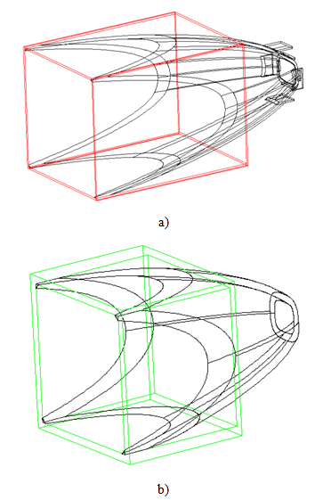Figure 29. CAD model of Rondine Gen1 (a) and Rondine Gen2 (b) after the addition on the front aperture of four planar ideal mirrors. The two prototypes are shown with a different scale

We suppose (this assumption is reasonable because an high efficiency solar cell has a quite isotropic surface) that the behaviour of the solar cell used as receiver is independent on the orientation of the plane of incidence, i.e. on the azimuthal angle β. As a consequence, we measure the distribution of the flux incident on the cell, that is of the flux transmitted by the open exit aperture of the Rondine, as function of only the polar emission angle (α).

We have that the total flux incident on the solar cell (CELL mode), Φ_INC (θ, φ), is equal to the flux transmitted by the Rondine when the exit aperture is open (SPHERE mode), (see also Fig. 5):

(13)

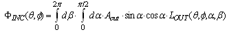
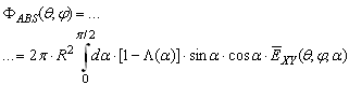
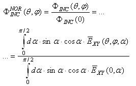
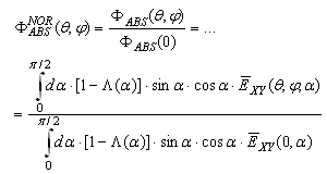
where is the radiance of the light emitted from the exit opening. The flux Φ_INC(θ, φ) can be expressed as function of the irradiance measured on the hemispherical screen (see Section 5.6), E_SCREEN (θ, φ, α, β):

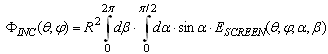(14)

The irradiance E_SCREEN (θ, φ, α, β), when projected over the x/y plane, orthogonal to the optical axis, gives E_XY (θ, φ, α, β). Eq. (14) then becomes:

(15)

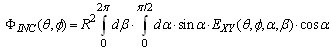
As we are interested only to the α-dependence, we average E_XY (θ, φ, α, β) over angle β, setting the rotational symmetry of that function and obtaining the β-symmetrized function . The flux Φ_INC(θ, φ) now becomes:

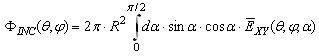(16)

To know the effect that the angle of incidence of light has on the absorption properties of the Rondine solar cell, we need now to simulate the total flux absorbed by the solar cell (CELL mode), Φ_ABS(θ, φ), by introducing the relative loss function, Λ(α), calculated before (see Eq. (11)):

(17)

We now normalize the total incident flux of Eq. (16) to the total flux incident at 0° and the total absorbed flux of Eq. (17) to the total flux absorbed at 0°:

(18)

(19)

The angle resolved normalized total flux of the Rondine Gen1 incident on the solar cell, that is transmitted without loss to the output, and simulated by Eq. (18), corresponds to the transmission efficiency curves of the Rondine Gen1 measured in the SPHERE mode (see Figs. 23, 24). The angle resolved normalized total flux of the Rondine Gen1 absorbed by the solar cell, equivalent to the normalized short circuit current of the solar cell, than transmitted with loss to the output, and simulated by Eq. (19), corresponds to the transmission efficiency curves of the Rondine Gen1 measured in the CELL mode (see Fig. 25).

We have simulated the function of Eq. (18) and the function of Eq. (19) for the x-axis (φ = 0; long edge of the exit aperture) of the Rondine Gen1. They are reported in Fig. 30.

Figure 30. Normalized angle-resolved transmission efficiency of the Rondine Gen1 along the x-axis (φ = 0), obtained simulating the DCM method with the SPHERE (star dots) and CELL (circle dots) receiver

For the function we measure an acceptance angle of 4.5±0.2° at 90% of 0° efficiency and 8.3±0.2° at 50% of 0° efficiency. For the function we measure an acceptance angle of 4.3±0.2° at 90% of 0° efficiency and 8.2±0.2° at 50% of 0° efficiency. The two functions and are practically overlapping and no shrinkage of the curve is observed; this means that the effect of the angle of incidence of light focused from Rondine Gen1 on the solar cell is negligible and does not alter the shape of the curve compared to the curve. 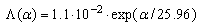This behaviour is expected also for and (y-axis), because the Λ(α) function is the same for the two azimuthal orientations. This confirms our assumption that the optical loss (narrowing of the transmission efficiency curve) associated with the transition from the SPHERE to the CELL mode operation, does not depend on the optical loss of the bare solar cell, and then must be sought elsewhere. Watching carefully the status of receiver in the Rondine Gen1, we noticed that the coupling between the concentrator and the solar cell is not optimal. In fact, for the characterization work, we used as receiver a bare solar cell, the same mounted in the module, but without encapsulation and just placed faced to the exit opening. The result is that the active area of the cell does not completely fill the exit opening, so part of light is lost at the periphery of the cell, causing the reduction of the transmission efficiency, as observed experimentally (see Fig. 25). The fact is illustrated in Fig. 31, where it is shown the detail of the receiver in the Rondine Gen1. The bus bars affect mainly the y-axis operation of the concentrator, as they are exposed to the concentrated light in the upper and lower part of the receiver; also the x-axis is affected by the slightly shorter length of the cell respect to the exit opening. We expect therefore to have shrinkage of the efficiency curve along both the x-axis (long edge of exit aperture) and y-axis (short edge of exit aperture), as it was effectively observed (see Fig. 25).

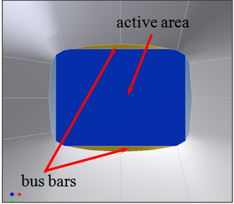Figure 31. a) Particular of the solar cell with the horizontal (x-axis) bus bar of the grid; b) The bus bar appears slightly exposed at the exit opening of the Rondine Gen1

The effect of the non-optimal matching of the concentrator with the solar cell has been simulated by tracing the curve of efficiency along the x-axis for two types of solar cells (both imagined perfect absorbers): the real cell with the size of the one used in the CPV module, and an optimised cell that completely fills the exit opening of the Rondine. The results are shown in Fig. 32. The two normalized efficiency curves are significantly different. The curve of the optimised cell presents the following acceptance angles: = 4.5±0.2°, = 8.3±0.2°, whereas the curve of the non-optimised cell presents the following acceptance angles: = 3.2±0.2°, = 6.6±0.2°. These results are consistent with what obtained experimentally by operating, respectively, in the in SPHERE mode (ideal absorber = optimised cell) and in the CELL mode (non-optimised real cell).

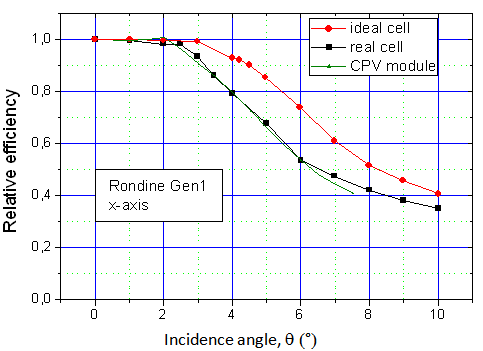Figure 32. Normalized angle-resolved transmission efficiency of the Rondine Gen1 along the x-axis, obtained simulating the DCM method, and using two different cells (as ideal absorbers): a cell of reduced dimensions (black curve); a cell with optimised dimensions (red curve). For comparison, it is reported the normalized “electrical” efficiency curve of the Rondine CPV module (green curve)

An interesting result is obtained comparing the simulated “optical” efficiency of the Rondine Gen1 + real cell with the electrical (power) efficiency of the corresponding CPV module. The two curves are normalized and shown in Fig. 32. They are practically coincident, demonstrating that so far our simulations and interpretation of results is correct and that the angle-resolved “optical” behaviour of the Rondine + cell concentrator is the same of the angle-resolved “electrical” behaviour of CPV module. The current configuration of the CPV module Rondine Gen1 is outlined in Fig. 33. The solar cells are encapsulated within an anti-corrosion glass plate (gl) with a thickness of 1 mm.

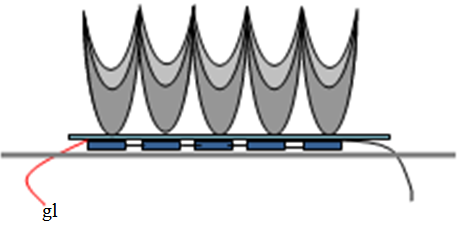Figure 33. Schematic section of a small region of the Rondine Gen1 CPV module

A final consideration to do is that, by acting on the receiver and optimising the matching between Rondine Gen1 and cell, it is possible to retrieve the optical acceptance angle measured in the SPHERE mode and to transfer it in the CPV module.

Experimental measurements by the DCM method were carried out also on the Rondine Gen2 concentrator. We used the configuration B and the SPHERE receiver.

Fig. 34 shows the normalized curve of optical efficiency along one axis parallel to the edge of the input aperture (x-axis and y-axis are here optically equivalent).

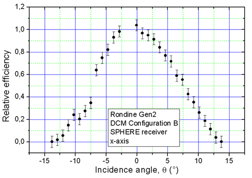Figure 34. Experimental normalized efficiency of Rondine Gen2 traced with the DCM, configuration B, and SPHERE receiver

The measured acceptance angles are: 3.6±0.5° at 90% of 0° efficiency and 7.4±0.5° at 50% of 0° efficiency. The data are affected by high random errors due to the very low signal on the photodetector.

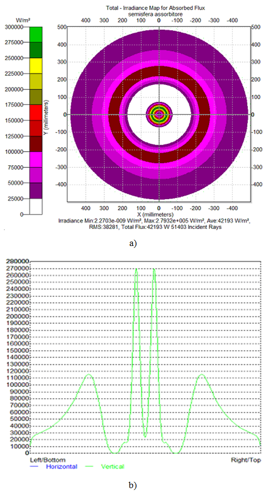
5.2. Transmission Efficiency by the Inverse Method

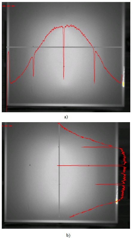
We discuss here the results of the experimental measurements made by ILM on the Rondine Gen1. The schematic of the experimental apparatus is that reported in Fig. 16. Fig. 35 shows the three-dimensional irradiance map produced on the screen. It represents the quantity E_C (θ, φ) introduced in Section 4. It has an elliptical form, reminiscent of the exit opening of rectangular shape. By using HiPic, we drew the horizontal and vertical profiles of the irradiance on the screen (see Fig. 36). Differently from the calibration profiles of Fig. 20, these profiles were traced centering the inverse image and avoiding the black dots. Normalizing E_C (θ, φ) and applying Eq. (8), we finally obtain the normalized radiance , equivalent to the normalized efficiency (see Eq. (9)).

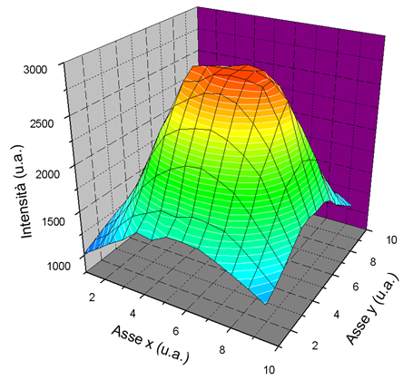Figure 35. Three-dimensional view of the irradiance map produced on the screen by the inverse light from Rondine Gen1

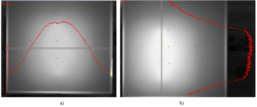Figure 36. Analysis by HiPic of the ILM image produced by Rondine Gen1. The irradiance profiles (red lines) are traced along the horizontal (x-axis) (a) and vertical (y-axis) (b) directions

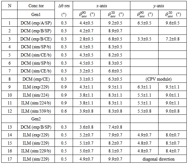
The normalized efficiency has been calculated for two crossed azimuthal directions, the horizontal (x) and vertical (y) axes, parallel to the edge of input aperture, and are shown in Fig. 37.

The measured acceptance angles are: 4.3±0.2° (x-axis) and 6.3±0.2° (y-axis) at 90% of 0° efficiency and 9.5±0.2° for both axes at 50% of 0° efficiency, in good agreement with the experimental results of direct method configuration A (see Fig. 23) and configuration B, SPHERE receiver (see Fig. 24).

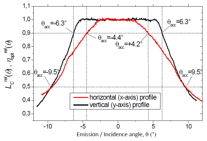Figure 37. Experimental relative radiance vs. emission angle, or transmission efficiency vs. incidence angle, of Rondine Gen1, traced along the horizontal and vertical axes, with the ILM method at d = 229 cm

The ILM results for the Rondine Gen2 prototype, obtained by a concentrator-screen distance d = 224 cm, are reported in Fig. 38. Rondine Gen2 has a quasi-squared exit aperture, then we expect equal efficiency profiles for the x and y azimuthal directions. The two curves of radiance, or optical efficiency, indeed, are virtually overlapping and show similar acceptance angles: 5.2±0.2° (x-axis), 4.9±0.2° (y-axis) at 90% of 0° efficiency and 7.9±0.2° (x-axis), 8.0±0.2° (y-axis) at 50% of 0° efficiency.

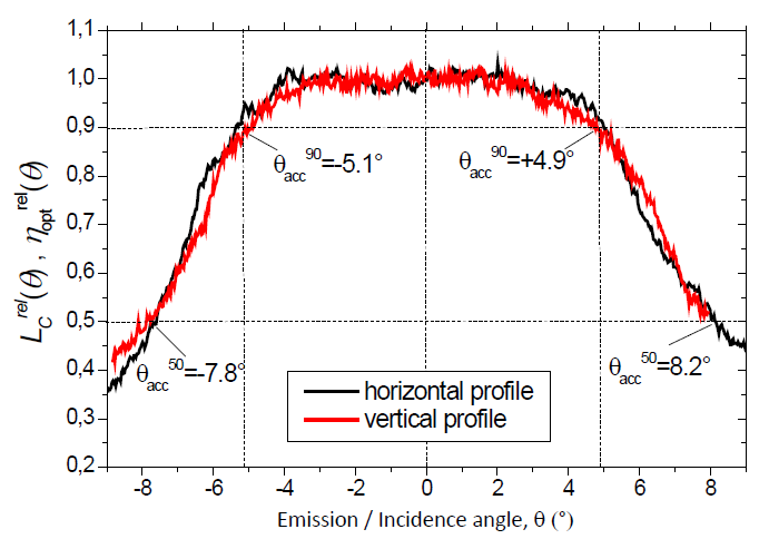Figure 38. Experimental relative radiance vs. emission angle, equivalent to transmission efficiency vs. incidence angle, of Rondine Gen2, traced along the horizontal and vertical axes with the ILM method at d = 229 cm

The first optical simulations with the ILM method were devoted to verify that the optical efficiency of Rondine Gen1 was not changing adding the side box at entrance, as mentioned in section 5.1.

This is shown in Fig. 39, where the efficiency curves along the x-axis and y-axis are drawn. It can be observed that only for very high polar angles (>15°) a slight difference is observed between the transmission efficiency curves. The curves of Fig. 39 refer to a distance between screen and concentrator, d =224 cm. According to Eq. (6), this means an angular resolution of around 0.9°. The measured acceptance angles are: 3.8±0.2° (x-axis) and 5.5±0.2° (y-axis) at 90% of 0° efficiency and 8.3±0.2° (x-axis) and 9.0±0.2° (y-axis) at 50% of 0° efficiency. A resolution better than 0.6° is achieved by working with a screen at a distance d =339 cm. The simulated ILM relative inverse radiance of Rondine Gen1, simulated at d =339 cm and drawn along the x and y axes, are shown in Fig. 40.

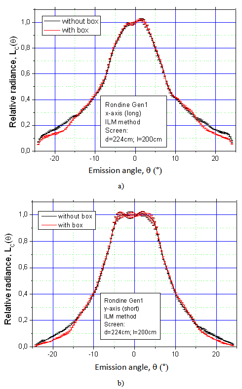Figure 39. Relative angle-resolved radiance of emission of the Rondine Gen1 irradiated by the ILM method, traced along the x-axis (a) and the y-axis (b), with (red line) and without (black line) the box at the input aperture

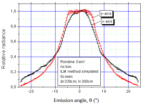Figure 40. Relative angle-resolved radiance of emission of the Rondine Gen1 without side box, irradiated by the ILM method, traced along the x-axis (dark line) and the y-axis (red line)

The measured acceptance angles are: 3.9±0.2° (x-axis) and 5.5±0.2° (y-axis) at 90% of 0° efficiency and 8.3±0.2° (x-axis) and 9.0±0.2° (y-axis) at 50% of 0° efficiency. The errors attributed to angle are derived from the limit number of rays used in the simulations, and then they are to be considered as statistical errors, whereas the angular resolution calculated by Eq.s (5) or (6) establishes the upper limit to the angle precision in absence of statistical errors.

The ILM simulations on the Rondine Gen2 with and without box were carried out at a Rondine-screen distance d = 229 cm, the same used in the experiments (see Fig. 38).

The map of irradiance E_C (θ, φ) obtained on the screen (ps) (see Fig. 16), as a result of a 500k ray-tracing process, is shown in Fig. 41 for the Rondine without box. It is interesting to observe how the symmetry of the map changes with distance from the centre, i.e. with the angle of emission. The symmetry is circular near the centre, then becomes squared with axes parallel to those of the Rondine edges, then returns to be circular and finally becomes squared again with a rotation of 45° respect to before. This changes of symmetry is consequence of the particular shape of Rondine wall, alternating between square and quasi-circular symmetry. From the irradiance map we have extracted the profiles , normalized as and finally transformed into the relative radiance following Eq. (8). 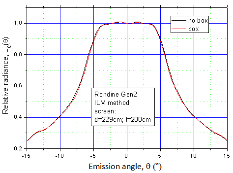The radiance profiles, equivalent to the transmission efficiency , extracted for the x and y directions overlap very well, demonstrating the accuracy of the optical fabrication process of Rondine Gen2. The measured acceptance angles are: 5.1±0.2° (x-axis) and 4.8±0.2° (y-axis) at 90% of 0° efficiency and 8.2±0.2° (x-axis) and 8.5±0.2° (y-axis) at 50% of 0° efficiency, in good agreement with the experimental results. The inverse radiance was simulated also for the Rondine Gen2+box and the resulting curves, averaged over the x and y-axes, are compared in Fig. 42. Fig. 42 shows that the real Rondine Gen2 concentrator, whose side planar walls were removed (see Fig. 2), behaves exactly as it had the same walls as ideal mirrors.

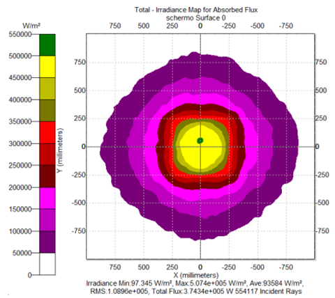Figure 41. ILM map of irradiance produced on the planar screen by the inverse light from Rondine Gen2 (no box) at d = 229 cm

Figure 42. Simulated inverse radiances vs. emission angle of Rondine Gen2, with and without box, averaged over the x and y directions, with the ILM method at d = 229 cm

This result justifies the choice of removing the sidewalls, which, also in the best real case, would never be equivalent to two ideal reflectors.

The map of Fig. 41 leads us to another consideration. The Rondine Gen2 module is actually oriented in such a way to track the Sun disk along the x or y-axis (they are equivalent in Gen2). Angular misalignments between Gen2 and Sun are then expected along that direction. The map of Fig. 41, however, seems to favour the diagonal direction, instead of the x/y one. If we calculate the inverse radiance curve along the diagonal direction, indeed, we find that it is wider than that calculated along the x/y axis, as shown in Fig. 43. We have in fact: x/y direction: ≈ 5.0±0.2°, ≈ 8.4±0.2°, diagonal direction: = 4.9±0.2°, = 9.9±0.2°.

Then, in order to increase the collection capability of the Rondine Gen2 along the direction of tracking, it could be convenient to have the tracking direction parallel to the diagonal of the opening entrance. This is valid for misalignments >, because, as it can be seen in Fig. 43, is improved of ≈ 20%, but remains constant.

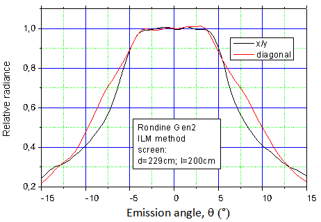Figure 43. Simulated inverse radiances vs. emission angle of Rondine Gen2, calculated along the x/y direction and along the diagonal direction, with the ILM method at d = 229 cm

All the optical and electrical results of acceptance angle discussed until now for the Rondine concentrators are summarized in Table 1.

Table 1. Results of acceptance angle (in degree) (exp = experimental; sim = simulated; A = configuration A; B = configuration B; SP = SPHERE; CE = CELL; PW = Power; xxx = d (cm) Rondine–screen distance; b = box). The results are reported with the same order as they appear in the text

The acceptance angles are reported with a cumulative error given by the sum of the statistical error and the angle resolution Δθ_res given by the intrinsic angular indeterminacy of the used method. Δθ_res is reported in a separate column in Table 1.

From Table 1, combining the results of DCM and ILM, doing the weighted average of the experimental and simulated values, and assuming an ideal receiver, we get for the acceptance angles of the two Rondine concentrators the most probable values reported in Table 2.

Table 2. Summary of the results given in Table 1 for Rondine Gen1 and Gen2 concentrators with an ideal receiver

As regards the measures of transmission efficiency of the two Rondine prototypes, we can summarize as follows the results exposed above:

i) The results of Table 1 show, first of all, that the DCM and ILM methods are equivalent within the experimental or simulated errors.

ii) DCM, using an integrating sphere equipped with a photodetector as receiver, gives the optical efficiency of the concentrator itself, while the direct use of a solar cell as receiver gives the optical efficiency of the whole system: the photovoltaic concentrator.

iii) The use of DCM by a particular cell as receiver (the one with the exposed bus bars) resulted in the narrowing of the transmission efficiency curve.

iv) The power curve of the CPV module gives an efficiency curve equal to that obtained with the use of the cell with the exposed bus bars.

v) The DCM and ILM methods give the same values of acceptance angles when the DCM method is applied with an ideal receiver.

We are finally able to give some results of on-axis absolute efficiency , obtained experimentally. The on-axis front image of Rondine Gen1 input aperture is shown in Fig. 22. It is clearly visible the central rectangular region of the receiver (the exit aperture). The radiance of the receiver in Fig. 22 is slightly underestimated due to the presence of the baffle at the centre (see Fig. 19b). By correcting this effect, we obtain a better estimate of which, together with the average radiance of the whole image, gives = 84.0±1.0% (see Eq. (10)). For the Rondine Gen2 concentrator we obtain = 86.0±1.0%.

5.3. Flux Distribution on the Receiver

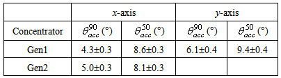
The analysis of the spatial distribution of output flux from a PV concentrator is important because of its strong influence on the conversion efficiency [39, 50-53]. As it has been demonstrated in previous works [7, 38], a canonical 3D-CPC, aligned with the Sun, presents an unacceptable flux distribution, mainly focused on the optical axis. To work around this problem, the Rondine concentrator, belonging to the class of the light cones, was obtained modifying a 3D-CPC as follows: by truncating it, deforming the lateral surface, squaring the entrance opening and finally removing the lateral walls (see Fig. 2). The effect of this CPC redesign is the mixing of rays and a better distribution of flux, particularly when the Rondine is aligned with the Sun (θ = 0°). We start considering the Rondine Gen1. Fig. 44 shows the simulated maps of irradiance on the receiver at different angles of incidence of a collimated beam in direction of the x-axis.

Fig. 45 shows other simulated maps for the collimated beam bent at different angles towards the y-axis. Fig. 46 shows some simulated maps of irradiance on the receiver for the Rondine Gen2. From Figs. 44-46 we see, first of all, that the output flux is distributed well on the receiver when the Rondine is aligned with the Sun; in addition, the flux distribution affects the entire surface of the receiver even for angles of incidence within the acceptance angle . The geometry of the two Rondine concentrators, therefore, does not require a secondary mixer, normally used in combination with a cone of light as a CPC.

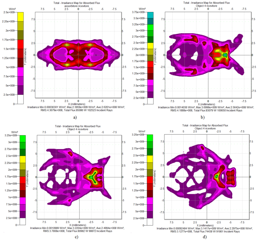Figure 44. Maps of irradiance of Rondine Gen1 output flux at some incidence angles of the collimated beam along x-axis: 0.0° (a), 2.0° (b), 3.0° (c), 4.0° (d). Number of input rays: 100k

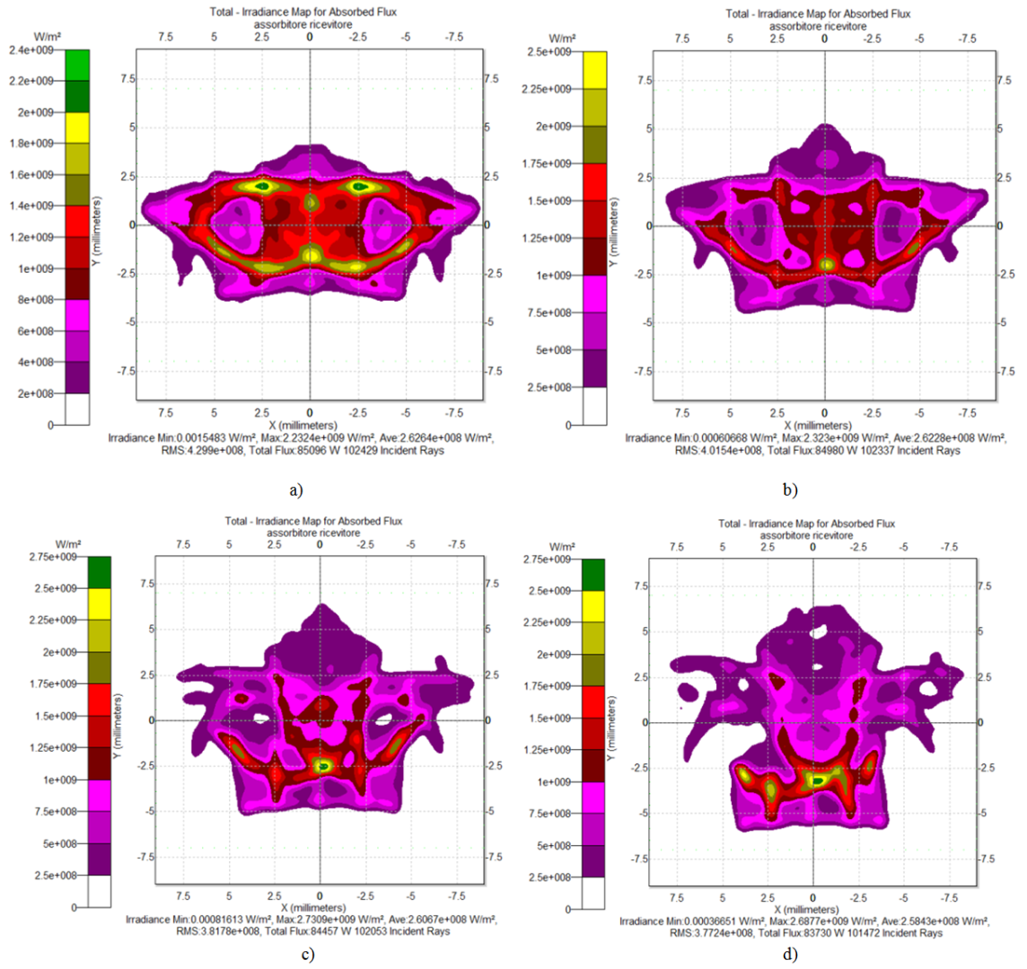Figure 45. Maps of irradiance of Rondine Gen1 output flux at some incidence angles of the collimated beam along y-axis: 1.0° (a), 2.0° (b), 3.0° (c), 4.0° (d). Number of input rays: 100k

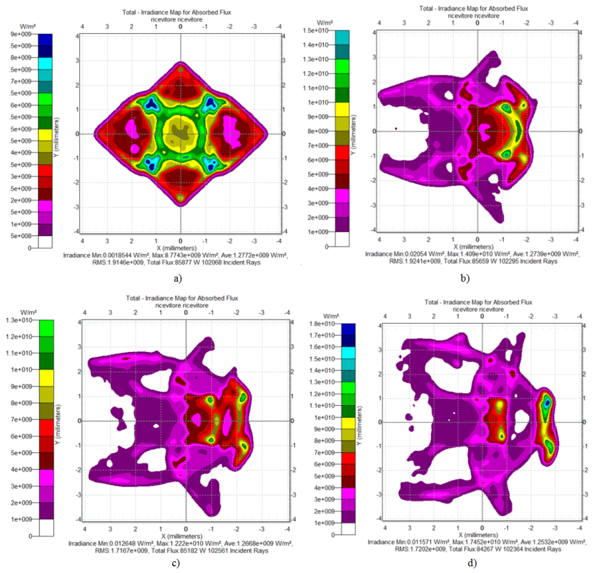Figure 46. Maps of irradiance of Rondine Gen2 output flux at some incidence angles of the collimated beam: 0.0° (a), 2.0° (b), 3.0° (c), 4.0° (d). Number of input rays: 100k

5.4. Number of Reflections of Transmitted Rays

In an ideal 3D-CPC concentrator, the average number of reflections is low and almost constant with the incidence angle within [7]. In the case of Rondine concentrator, the length was defined to obtain about only one reflection for the entering rays parallel to the optical axis, to reduce the optical losses by multiple reflections. The procedure used by us to estimate the average number of reflections of the transmitted rays of a collimated beam incident at different angles is discussed in a previous work [7]. Here we simply bring the final formula:

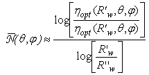(20)

where: R'_w e R''_w are two arbitrary values of specular reflectance close to the true value of wall reflectance, η_opt is the optical efficiency and is the average number of reflections. To apply Eq. (20), we have carried out a fast series of DCM simulations to get the optical efficiency of Rondine vs. the polar angle for reflectances R'_w = 0.83 and R''_w =0.87, close to the specular reflectance of Rondine R_w = 0.85 (see Section 2).

Fig. 47 shows that the average number of reflections is equal to one at the optical axis, as expected, then grows and reaches a maximum at around , as it was also found with an ideal 3D-CPC [7].

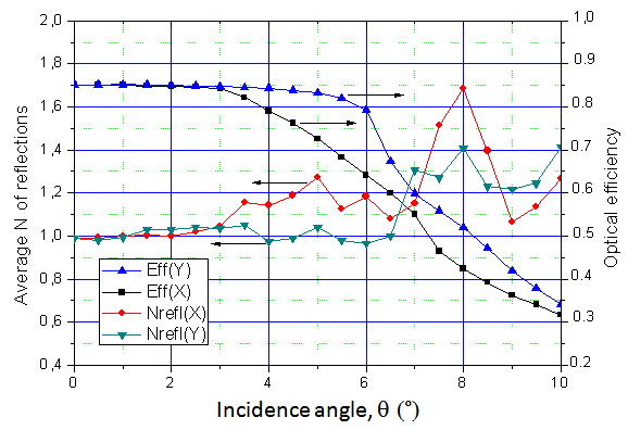Figure 47. Simulated curves of absolute optical efficiency of Rondine Gen1 and corresponding curves of average number of reflections obtained by applying Eq. (20). The curves refer to x and y-axes

In any case, maintains always very near to one below the acceptance angle . The optical efficiency at 0° is ~0.85, the same value of the specular reflectance R_w, as required for one reflection. This result agrees with our previous on-axis ILM measurements on Rondine Gen1: = 0.84±0.01 (see last part of Section 5.3) and represents therefore a further validation of ILM method.

Fig. 48 shows the results of average number of reflections for the Rondine Gen2. is now slightly lower than one on the optical axis, effect of the lower concentration ratio of Gen2 respect to Gen1 (see Fig. 3) and of the stronger deformation of the Gen2 geometry respect to the canonical CPC, which reduces multiple reflections of rays near the edges of input aperture [7]. shows a monotonic growing with θ, without a maximum at the acceptance angle as observed in Gen1, probably as a further cause of its strong differentiation from the ideal CPC geometry.

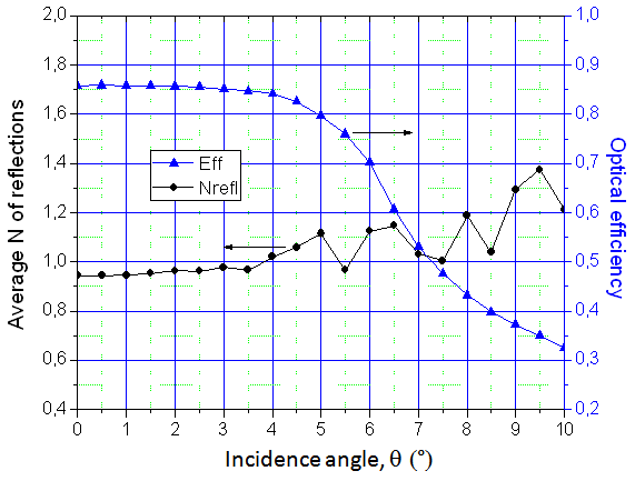Figure 48. Simulated curve of absolute optical efficiency of Rondine Gen2 and corresponding curve of average number of reflections obtained by applying Eq. (20)

The optical efficiency at 0° is ~0.86, and agrees very well with our previous on-axis ILM measurements on Rondine Gen2: = 0.86±0.01 (see last part of Section 5.3).

5.5. Angular Distribution of the Transmitted Flux

To study the angular distribution of the transmitted rays, we have coupled the Rondine with a hemispherical screen, of internal radius R, whose inner wall has been set as an ideal absorber, making coincide the centre of the exit aperture of Rondine with the centre of the hemispherical screen (see Fig. 49).

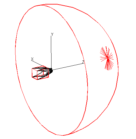Figure 49. Layout of the configuration used for the simulation of the angular distribution of light transmitted by the Rondine Gen1

When the Rondine Gen1 is irradiated with the DCM method by the parallel beam, we change the polar angle θ and maintain fixed the azimuthal angle φ corresponding to the orientation of the plane of incidence that we have fixed parallel to one of the two edges of the input aperture shown in Fig. 29, also distinguished as x-axis (parallel to the long edge of the exit aperture) and y-axis (parallel to the short edge of the exit aperture).

The rays are transmitted from the exit aperture along the polar angle α and the azimuthal angle β. The transmitted beam, characterized by the radiance L_OUT (θ, φ, α, β), is absorbed by the screen and produces the irradiance E_SCREEN (θ, φ, α, β). This irradiance is projected on the x/y plane orthogonal to the optical axis, producing the irradiance E_XY (θ, φ, α, β).

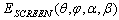An example of the 3D map of irradiance function obtained irradiating the Rondine Gen1 by DCM is shown in Fig. 50. As we are interested to study the distribution of output flux as function of only the polar angle α, we transform the irradiance E_XY (θ, φ, α, β) in the β-symmetrized function by setting the rotational symmetry. Fig. 51 shows an example of rotational map and the corresponding radial profile. The radial profile of Fig. 51b is plotted as function of r, distance of the projected point on the screen from the optical axis; then we have: sinα = r / R, with R screen radius.

Figure 50. Rondine Gen1 3D map of the irradiance produced on the internal surface of the hemispherical screen

Figure 51. Rondine Gen1 map of the β-symmetrized irradiance projected on the XY plane (a) and corresponding radial profile for θ=5° incidence along the y-axis (φ =90°) (b)

The βsymmetrized function corresponds to the output radiance of Rondine, , after β-symmetrization: . We can write therefore for the elemental flux in the α, α+dα interval:

(21)

from which we have for the angular density of the output flux:

(21)

The function has been simulated for the Rondine Gen1 along the x-axis (φ = 0) and the y-axis (φ= 90°), for α varying in the 0°÷10°, and the results are shown in Fig. 52. Figs. 52a and 52b show that, apart from a minor peak near 0°, in the Rondine Gen1 most of the outgoing flux has a divergence between about 20° and 80°, with a large peak at around 30° which tends to move to the right at increasing the input incidence angle.

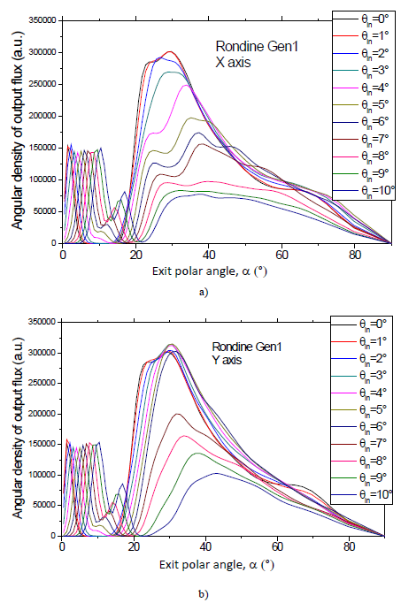Figure 52. Angular density distribution of the output flux transmitted by the Rondine Gen1 (+box) as function of ten incidence polar angles of the parallel beam at input: θin = 0.0°-10.0° with steps of 1.0°. (a) The beam is oriented towards the x-axis (φ =0°). (b) The beam is oriented towards the y-axis (φ =90°)

We observe also that, at increasing the input incidence angle, the output flux is better distributed over the half-space. These angular distribution conditions are very favourable for photovoltaic applications, because most of the flux is contained in the range 20°-60°, which is not too high to require exceptional light collection performances from the used solar cell.

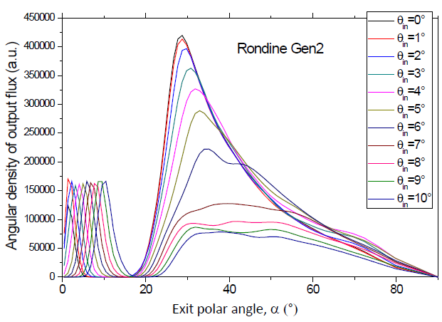Figure 53. Angular density distribution of the output flux transmitted by the Rondine Gen2 (+box) as function of ten incidence polar angles of the parallel beam at input: θin = 0.0°-10.0° with steps of 1.0°

6. Conclusions

We have described two methods for the optical analysis of light concentrators with a detailed characterization of two specific nonimaging concentrators already employed in low concentration photovoltaic module. The first presented technique is a conventional “direct” method (DCM) which simulates the direct solar irradiation; the second one is the recently developed “inverse” method (ILM) where the concentrator is reversely used as illuminator, applying a proper extended light source at the exit aperture of the concentrator. We have demonstrated the equivalence between the two methods to get the angle-resolved optical efficiency of the optics by experimental and simulated measurements. We have also demonstrated that ILM is significantly more advantageous than DCM when dealing with small size concentrators, in terms of handiness and operating speed. Besides the measurements of optical transmission efficiency, we report the results of simulations for other relevant parameters characterizing the optics: the average number of the light-rays’ reflections on the reflective wall of the concentrator under test; the spatial flux distribution on the receiver; the angular distribution of light at the output of the concentrator.

Analysing these results, we can conclude that the “Rondine^®” light concentrators here evaluated show optical properties appropriate for CPV applications. In particular, the following points are particularly relevant: high optical efficiency when the concentrator is well aligned toward the Sun; high acceptance angles, which allow the use of these concentrators on two-axis PV solar trackers with pointing accuracy within ±4°; absence of hot-spots on the receiver, thanks to an adequate spatial and angular distribution of the light flux at the output of the concentrator.

ACKNOWLEDGMENTS

We acknowledge with gratitude the help provided by dott. Mauro Campa during the experimental measurements on the Rondine.

Appendix

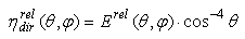
When the inverse method is simulated, the planar screen is configured as an ideal absorber and the profile of the measured incident irradiance (see Fig. A1a) is converted into the profile of the radiance distribution function of the concentrator, , by the (cosθ)^-4 factor. Indeed, if is a point on the screen, the corresponding incident irradiance and dS an elementary area around , the flux through area dS is 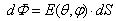and it is confined within the solid angle given by:

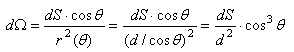(A1)

The inverse radiance produced by the concentrator towards direction will be therefore expressed by:

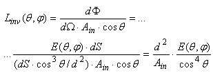(A2)

where A_in is the input aperture area of concentrator. The radiance can be normalized to the value at θ = 0° giving:

(A3)

The inverse radiance is related to the optical efficiency of the concentrator in the following way:

(A4)

We conclude that, when we simulate the inverse method, the normalized profile of the direct transmission efficiency of the concentrator is directly derived by the normalized irradiance incident on the ideal absorbing screen, by the expression:

(A5)

When the “inverse” method is applied experimentally, the screen is used to send back the diffuse, inverse light towards the CCD and must have a Lambertian character (reflectivity independent on the incidence angle, and constant radiance of the reflected light, as function of observation angle) in order to allow the reconstruction of the irradiance map on the screen from the intensity map produced on the CCD.

If the CCD is aligned with the optical z axis and close to the concentrator (see Fig. A1b), the intensity profile of CCD image must be corrected by a further (cosθ)^-4 factor, as we demonstrate in the following (see also Fig. A1c).

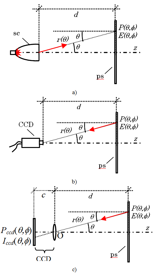Figure A1. (a) Schematic of the irradiation of the planar screen (ps) by the inverse light produced by the solar concentrator (sc). (b) Process of recording by the CCD of the image produced by the irradiance map produced on the planar screen. is a point on the screen and is the corresponding incident irradiance. (c) The CCD is schematised as a lens and a plane representing the image sensor of the CCD; is a point and is the intensity (irradiance) on the CCD sensor

The total flux reflected by the unitary area of (ps) centered in is:

(A6)

where R is the reflectance of (ps), is the reflected irradiance, and is the radiance of the screen. The flux reflected by the unitary area of (ps) and flowing inside the solid angle by which the unitary area is seen by point is:

(A7)

This flux is the same reaching the CCD sensor area (c / d)² centered on point . The intensity of the CCD image at point , proportional to the irradiance incident at that point, is therefore:

(A8)

By using Eq. (A2), we obtain:

(A9)

From Eq. (A9) we finally obtain the inverse radiance of the concentrator from the intensity on the CCD:

(A10)

The normalized radiance becomes:

(A11)

Finally, from Eq. (A4) we obtain the normalized transmission efficiency of the concentrator:

(A12)