1. Introduction

The Japanese economy entered a long slump in the early 1990s, widely attributed to stagnant corporate investments. In the wake of the bubble economy, corporate investments declined dramatically and have continued to stagnate ever since. Fixed investments are recovered over a long period of time; thus, their profits cannot be predicted accurately outside of a world of perfect foresight. As fixed investments are uncertain, the choice of investment is determined by the accuracy with which its profitability can be predicted. The collapse of the bubble economy in Japan and the increased anxiety in the Japanese financial market has made determining future prospects more difficult. This uncertainty is playing a significant role in investment choices.

The relationship between investment and uncertainty has been theoretically investigated since the 1970s. Hartman (1972) and Abel (1983), among the first to study this problem, developed a theory whereby uncertainty did not reduce investment and firms took positive investment action when facing uncertainty. This proposition depends crucially on the convexity of the marginal revenue product of capital in the output price. On the other hand, McDonald and Siegel (1986) and Dixit and Pindyck (1994) detected leeway in the timing and irreversibility of investments and came to the opposite conclusion—that a firm holding the monopoly right to invest in a given project has the right to choose the timing of the investment. This right has the same characteristics as a financial call option. If a fixed investment is irreversible, the values of the option to invest, which includes waiting, will increase along with the degree of uncertainty about future profits. Therefore, the firm will not invest unless the value of investing exceeds the value of waiting. Consequently, uncertainty suppresses investment. Completely different conclusions were reached via these two theories on the relationship between uncertainty and investment, both of which depend on the assumptions of a theoretical model. Empirical studies should therefore be conducted to determine which theory is more accurate. To complement the survey of empirical studies in Lensink et al. (2001), we discuss the key studies below. Pindyck and Solimano (1993) found that uncertainty over the marginal returns of capital had negative effects on investment based on cross-country data, and Ferderer (1993) indicated that uncertainty over the risk premium of interest rates had a negative influence on U.S. fixed investment. Moreover, Huizinga (1993) found that uncertainty over inflation rates and real wages had negative effects on U.S. fixed investment. Evidence from the current studies indicates that there is a negative relationship between uncertainty and investment.

Beyond the studies cited above, which were empirical and used macro data, research on the relationship between uncertainty and investment began to develop when the heterogeneity of the economic unit was considered using data from major industries or from individual firms. Leahy and Whited (1996) tested the impact of the substitutability between labor and capital on the investment–uncertainty relationship. Guiso and Parigi (1999) studied the investment behaviors of Italian firms and found that the competitive position of a product market varied among industries. They indicated that the negative effects of demand uncertainty on investment in industries with low market competition were smaller than those in industries with high competition. Pattillo (1998) investigated firms in Ghana and reported that irreversibility varied according to the type of capital equipment. She used the ratio of the real sales value of the capital stock to its real replacement value as an indicator of investment irreversibility and found that the negative effects were greater for groups of firms with more irreversible capital goods. Cassimon et al. (2002) investigated Belgian firms and measured the flexibility of capital equipment according to whether it had been leased. They showed that uncertainty was strongly and negatively linked to investment in a group of firms with no equipment flexibility.

However, few empirical studies have investigated how uncertainty affects firm investments in Japan. Two relevant studies—by the Economic Planning Agency (1993) and Matsubayashi (1995)—have used macro data. The Economic Planning Agency employed the forecasting error of the stock price to measure uncertainty, and Matsubayashi (1995) used the fluctuations in Tobin’s q. They both indicated a negative relationship between uncertainty and investment in Japan.

Ogawa and Suzuki (2000) and Suzuki (2001) conducted empirical studies using data from individual firms. Ogawa and Suzuki (2000) performed a panel study relying on data from a manufacturing firm and found a significantly negative relationship between uncertainty and fixed investment. They also estimated the investment function using the cross-product of the uncertainty measure with a dummy variable taking unity for firms in the materials industry group (i.e., chemicals, iron and steel, and non-ferrous materials and products) and found that the cross-term was significantly negative. They concluded that, since tangible assets depreciated more slowly in the materials industry group than in the machinery industry group and as the speed of depreciation was negatively correlated with the degree of asset specificity (i.e., sunk costs), the results were perfectly consistent with the theory that the negative relationship between uncertainty and investment depends on the degree of irreversibility. Suzuki (2001) extended their analysis by examining the investment–uncertainty relationship with a focus on the heterogeneity between the materials and machinery industries. Considering the size of a firm in conjunction with the abovementioned factors, he found that the negative relationship between investment and uncertainty in the materials industry was strong in large firms and that the negative relationship of the machinery industry was strong in medium-sized firms, which included a few mid-rank firms. Thus, these two studies focused on the heterogeneity among industries and showed that uncertainty’s effect on fixed investment differs according to the industry and firm size. However, these studies did not examine the industrial characteristics involved in this relationship.

This paper examines the industrial characteristics related to the extent of uncertainty’s negative effects on investment using Japanese manufacturing data. We focus on the degree of competition in the product market and the degree of irreversibility.

The rest of this paper is organized as follows. Section 2 provides the theoretical background necessary for empirical studies on the uncertainty–investment relationship, following McDonald and Siegel (1986) and Dixit and Pindyck (1994), and presents two hypotheses. Section 3 describes the investment functions and constructs several measures of uncertainty. Section 4 interprets the estimates and verifies the hypothesis. Section 5 presents the study’s conclusions. Section 6 is a data appendix that explains the data used (with the exception of the measurement of uncertainty).

2. Theoretical Framework

2.1. Theoretical Background

Prior to the empirical study, Section 2 outlines the theoretical background of the relationship between investment and uncertainty, drawing from McDonald and Siegel (1986) and Dixit and Pindyck (1994). The adjustment cost function of investment is usually considered under the assumption that the adjustment cost for investing in plant and equipment is equal to that of disposing of capital equipment. It then follows that disused capital goods can be sold at a price that does not lose in a secondhand market. However, no perfect secondhand market for capital equipment exists. The sales value of capital goods improved to the users’ satisfaction and then sold to other firms is likely to fall. Thus, the adjustment costs of investing in plant and equipment and those of disposing of them are not symmetrical; the adjustment cost of disposing of capital goods is considerably higher than the costs at the time of purchase. Therefore, some of the capital investment may not be recoverable, making it irreversible.

When investment is irreversible, its timing becomes very important if the future prospect is uncertain. If it is assumed that a firm has the monopoly right to invest in a given project, it would not have to invest immediately. It would then be rational for the firm to invest when the uncertainty of the project’s profitability has lessened. If uncertainty lessens and the value of waiting to invest falls lower than the value of investing, the firm will invest in the project. Uncertainty therefore increases the rate of the expected earnings required for the execution of the option to invest and results in compressed investment. Accordingly, a firm’s investment opportunities include the right, but not the obligation, to purchase equipment at some future time. These rights to acquire real assets are called “real options.”

So far, we have considered a single and discrete project. However, firms usually hold two or more enterprises and invest in new additional projects: the investment decision is sequential. Dixit and Pindyck (1994) showed that their results did not change when the investment was sequential.

The argument so far has carried two constraints: (1) a firm has the monopoly right to invest, and (2) investment is completely irreversible. These two constraints will be eased and the conclusion re-examined. First, when the constraint under which a firm has the monopolistic right to invest is eased, the incentive to wait for an investment is reduced through the first-mover advantage effect under oligopoly conditions, as posited in Dixit and Pindyck (1994). As a result, the period for which an investment can be postponed is limited under oligopoly conditions. In theoretical terms, it is unclear whether the effect of the call option or that of the first-mover advantage is stronger; it depends on the characteristics of the competition, the kind of uncertainty, and the initial state.

Perfect irreversibility, as well as the condition of a perfect secondhand market, is also a very large constraint. Abel et al. (1996) argued in favor of a model that partially accepted reversibility and eased constraint (2)—in other words, assumed that investment is completely irreversible. At this point, not only the call option, the right to wait to invest, but also the put option, the right to wait to dispose of capital goods acquired through an investment, occurs. Therefore, when it is accepted that investment is partially reversible, the value of the call options is reduced by the value of the put options. The net effect of this depends on the degree of irreversibility. Since the value of call options is higher than that of put options with a high degree of irreversibility, uncertainty has more negative effects on investment.

2.2. Hypothesis

This paper empirically explains the relationship between uncertainty’s effect on fixed investment and industrial characteristics using a dataset of Japanese manufacturing firms. The industrial characteristics examined are the degree of competition in product markets and the degree of irreversibility of capital goods. We propose two hypotheses and discuss how the industrial characteristics affect the relationship between uncertainty and investment.

Hypothesis 1: Uncertainty has more negative effects on investment in an industry with low competition in market products than in one with high competition.

As shown in Section 2.1, the relationship between uncertainty and investment is not simple when market competition is considered. Under the assumption of imperfect competition, uncertainty’s effect on investment changes depending on the impact of the option (the right-to-wait investment) and the first-mover advantage.

Opposite results were obtained in empirical studies conducted by Ghosal and Loungani (1996) and Guiso and Parigi (1999). They tested the hypothesis that the effect of uncertainty on investment also changes according to the degree of competition in the products market. In an earlier study of U.S. manufacturing, a strong negative relationship between uncertainty and investment was observed with high competition in the products market. However, in a study on Italian manufacturing, a strong negative relationship was noted in an industry with low competition. More empirical studies will be necessary to determine which finding is correct. These results may show that the relationship of uncertainty and investment depends on the competitive condition of each industry in each country.

Hypothesis 1 is based on the following assumptions. If the degree of market competition is intense, the effect of the first-mover advantage will be strong, and the effect of the option (the right-to-wait investment) will be weak. In the state of perfect competition, the effect of the first-mover advantage completely reduces the value of waiting to invest. In such a case, the effects of negative uncertainty on investment are expected to be greater in an industry with low competition in the products market.

Hypothesis 2: Uncertainty has more negative effects on investment in an industry with high irreversibility than in one with low irreversibility.

When an investment is partially reversible, the value of the call option, the right-to-wait investment, is reduced by the value of the put option, the right to wait to dispose of the capital goods acquired through investment. This net effect depends on the degree of irreversibility of capital goods, and uncertainty has significantly negative effects on investment in an industry with high irreversibility.

In investment, all costs at the time of purchase are unrecoverable, even when capital equipment is no longer used despite being in working condition. Therefore, the degree of irreversibility of capital goods depends, for example, on the existence of secondhand markets for capital goods, the prices for used products, the existence of a rental market, and the possibility of diversion to other industries.

As mentioned, Ogawa and Suzuki (2000) estimated the investment function with the cross-product of the uncertainty measure with a dummy variable taking unity for firms in the materials industry group, determining that the cross-term was significantly negative. They concluded that the negative relationship between uncertainty and investment is strong in industries with high irreversibility because the life of tangible assets is longer in the materials industry group. However, it is not certain that the degree of irreversibility in the materials industry group was reflected in this estimation. Moreover, the life of tangible assets adopted as an irreversible measure is meaningful when there is no secondhand market for them. However, if the cost of the capital goods no longer used is completely recoverable in a secondhand market, the scale of the capital equipment and its lifetime will be unrelated to the degree of irreversibility. Therefore, the existence of a secondhand or rental market must be considered when examining the second hypothesis.

3. The Model and the Data

3.1. The Empirical Model

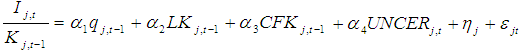
A set of panel data drawn from the financial statistics of listed firms is used to estimate the investment function with an uncertainty measure in this paper. The investment function is based on Tobin’s q, modified as described below to account for the characteristics of Japanese investment behavior.

Since the firm seeks the optimal path for its capital stock to maximize the expected present value of its net cash flow, Tobin’s q is the main explanatory variable. Furthermore, the financial factor, which is not taken into consideration in Tobin’s q theory, is added as an explanatory variable. The existence of asymmetric information between lenders and borrowers produces capital market imperfections and generates agency costs. The increased costs of capital accompanying the agency costs will affect investment. Two explanatory variables are added to account for that effect. One concerns the role of land used as collateral. This is used because firms’ borrowing constraints are reduced when land functions as collateral in cases where there is asymmetric information. Ogawa and Suzuki (1998) examined the relationship between borrowing constraints and land used as collateral employing data on Japanese firms. The other variable concerns the role of internal financing. If the agency cost is generated due to asymmetric information between lenders and borrowers and is added to the opportunity costs of internal financing as a premium, the firm will be released from such financing constraints. Furthermore, investment will be urged when internal financing is large. It is then possible to statistically examine whether uncertainty affects investment by adding the uncertainty measure to an explanatory variable other than these fundamental conditions. Thus, the basic investment function to be estimated is written as follows:

(1)

where

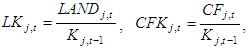I_j,t : real fixed investment of the jth firm in year t,

K_j,t : real capital stock of the jth firm at the end of year t-1,

q_j,t : Tobin’s q of the jth firm in year t,

LAND_j,t : land stock at market value of the jth firm at the end of year t-1,

CF_j,t : real cash flow of the jth firm in year t,

UNCER_j,t: measure of uncertainty of the jth firm in year t,

η_j,t : individual firm effect,

ε_j,t : disturbance term of the jth firm in year t.

Since investment and Tobin’s q are determined simultaneously in the theory, Tobin’s q in year t-1 of the right-hand side of formula (1) may be better to transpose than that in year t. Assuming that a time lag occurs between deciding on investment and capitalizing on the assets acquired through investment, Tobin’s q in year t may not be suitable as an explanatory variable. However, since a correlation arises between an error term and Tobin’s q in year t when formula (1) is estimated by the least-squares method, a consistent estimator may not be obtained. To ease such a simultaneous bias, Tobin’s q in year t-1 was used as an explanatory variable in this paper. Incidentally, the same result is obtained when formula (1) with Tobin’s q in year t is estimated by an instrumental variable method. The dependent variable is the investment rate, defined as the real investment divided by the real capital stock, and the land stock of a current price base and cash flow are divided by the real capital stock.

3.2. Sample Selection

The dataset is constructed from the database of the Development Bank of Japan, which contains financial report-based unconsolidated accounting data for companies listed on either the first or second sections of the Tokyo, Osaka, and Nagoya stock exchanges. We selected manufacturing firms that were active for more than 10 years from fiscal year 1977 to 2012. The sample thus includes data on firms newly listed and delisted. The data for firms that close their accounts in months other than March are placed in the fiscal years to which their accounting year-end months belong. Other studies exclude firms that change their fiscal years even once during the analytical period from the entire sample. To maximize our data, however, we have chosen to exclude from the sample only the period of that fiscal year and the following fiscal year. For mergers by listed firms, moreover, we did not sum the premerger numbers of both firms. They are excluded from the sample in the fiscal year of the merger and in the following year, and the pre- and post-merger firms are treated as entirely different firms. Firms that merged with unlisted firms or sold off their operating departments and split up were not deleted from the sample because they were very difficult to identify. These problems are controlled by removing outliers, as will be mentioned later.

Our analysis was undertaken on an unbalanced panel because the survival bias occurs: when analyzing on a balanced panel, only the firms that survive competition and maintain their listing are eligible. As the analytical data are limited to listed firms, that the sample is biased must be remembered when interpreting the estimation results for Japanese firms as a whole.

3.3. Measuring Uncertainty

In a theoretical model, uncertainty is usually included as a variable through a stochastic process. Since this uncertainty cannot be observed directly, it must be estimated by a specific method in empirical studies. The appropriate economic variable or method to use in measuring uncertainty is a matter of debate. Lensink et al. (2001) surveyed the uncertainty measurements adopted in empirical studies of investment and uncertainty. Ghosal (1991) built an uncertainty measure by computing a sample standard deviation of the numerical value of shipments in each industry. Ghosal and Loungani (1996) used the forecasting formation of the product price as the second-order auto-regression and made the standard error of an auto-regressive model the measure of uncertainty. Huizinga (1993) built an uncertainty measure using real wages and a product price through the general autoregressive conditional heteroskedastic (GARCH) model. Guiso and Parigi (1999) measured uncertainty using data obtained from a direct survey of future predictions employing a company questionnaire. Ogawa and Suzuki (2000), in developing an empirical study for Japan, built their uncertainty measure using the rate of change of real sales via three methods: conditional standard deviation, the standard error of an autoregressive model, and the ARCH model. Suzuki (2001) assumed that the value that discounted the average rate on equity by the cost of capital was a numerator of marginal q and used two methods to build an uncertainty measure—the conditional standard deviation and the standard error of an autoregressive model.

This paper focuses on the relationship between investment and the uncertainty of demand that firms face. The rate of change of real sales is adopted as the economic data that can be observed, similar to Ogawa and Suzuki (2000). Since Tobin’s q-type investment function is used for the estimation model, it was suggested that our uncertainty measure should also be built from Tobin’s q for the sake of model compatibility. However, since changes in sales are considered to be the most ambiguous component in Tobin’s q in terms of future prospects, changes in sales could be assumed to proxy for uncertainty.

Dixit and Pindyck (1994) divided uncertainty into the industry-level type, which all firms within the same industry face, and the firm-specific type, which each firm faces individually. Since output and price are determined endogenously, it is industry-level, rather than firm-specific, uncertainty that affects investment if the equilibrium of the whole industry is taken into consideration. We constructed our uncertainty measure from the sales growth rate of each firm and did not divide the uncertainty into two types. The uncertainty measure reported here includes each firm’s whole demand uncertainty.

We used a production deflator classified by the firms’ industry (Cabinet Office “Annual Report on National Accounts”) as a deflator to construct real sales. Three methods are used to measure uncertainty in this paper: the conditional standard deviation, the standard error of an autoregressive model, and the forecasting error of future prediction by an autoregressive model. Each method is described in detail below (please refer to the data appendix in Section 6 concerning data construction using a method other than the uncertainty measure).

3.3.1. Conditional Standard Deviation

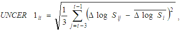
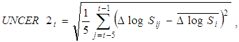
It is assumed that the standard deviation of the growth rate of the real sales computed for each firm is the uncertainty measure. Our assumption is that firms predict the growth rate of their following year’s sales by the average for the past several years and that the deviation from the average during that period is explained as the measure of the uncertainty of future predictions. It is difficult to determine how many previous years are important to consider. The previous five years are considered in Ogawa and Suzuki (2000), the previous three years in Suzuki (2001), and the previous five and ten years in Ghosal (1991). For this study, standard deviations from the previous three and five years were used as the uncertainty measure to establish the degree of robustness. UNCER1 is the conditional standard deviation of the real sales growth rate determined by using the previous three years, and UNCER2 is determined using the previous five years. They are formulated as follows:

(2)

(3)

where S_ij: real sales of the ith firm in year j.

The data series of the uncertainty measure was built for each firm by shifting this procedure by one year and repeating it.

3.3.2. Standard Error of the Autoregressive Model

The standard error of an autoregressive model was used as an uncertainty measure, as in Ghosal and Loungani (1996), Ogawa and Suzuki (2000). The assumption is that the prediction formation process of the growth rate of the following year’s real sales is expressed with an autoregressive model and that the standard error term of the regression is the measure of uncertainty. This study assumes that the growth rate of real sales is predicted based on the second-order autoregressive model (AR2) as follows:

(4)

where u_t: error term of the forecasting equation.

On the estimation of Equation (4), the rolling regression is applied to individual firms. To obtain the uncertainty measure for 2000, for example, Equation (4) is estimated for the period 1990–99, and the standard error of regression is obtained. The data series of the uncertainty measure is obtained by shifting this procedure year by year for each firm. When the uncertainty measure built by the above method is set to UNCER3, it is expressed as follows:

(5)

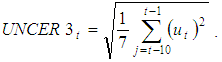
3.3.3. Forecasting Error of Future Prediction by Autoregressive Model

This method assumes that a firm predicts the future using past data and recognizes the deviations between predictions and actual data as uncertainty. This paper assumes that the growth rate of real sales is predicted based on the second-order autoregressive model expressed in Equation (4). The uncertainty measure for 2000 is taken as an example below, and the procedure used for the calculation is explained. First, Equation (4) is estimated for the period 1987–96. The 1997 growth rate of sales is predicted from the measurement result, and a deviation between the prediction for 1997 and the actual data is obtained. Next, the deviation between the prediction and the actual data in the 1998–1999 fiscal year is obtained by the same process. Finally, the numerical value—the square root of the average of the deviation squared for these past three years—is considered to be the uncertainty measure. When the uncertainty measure built by the above method is set to UNCER4, it is expressed as the following:

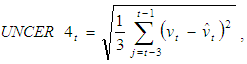(6)

where v_t: the actual data of Δlog S_t,

: Δlog S_t predicted on the basis of the second-order autoregressive model.

3.4. Data Description

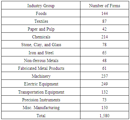
Although data from 1977 to 2012 are used, data for the 22 years from 1991 to 2012 are obtained through the data construction process described above. Only for UNCER4 do the data cover the 20 years from 1993 to 2012. Therefore, the model is estimated from 1991 to 2012. A total of 1,580 firms are analyzed. Detailed information on the sample firms is presented in Table 1. Among the three groups—materials (textiles, paper and pulp, chemicals, stone, clay, and glass, iron and steel, and non-ferrous metals), machinery (machinery, electric equipment, transportation equipment, and precision instruments), and others (foods, fabricated metal products, and miscellaneous manufacturing)—there were 534, 691, and 355 firms, respectively.

Table 1. Industry Classification and Number of Firms in the Sample

Abnormal values are removed from the data in the model estimation using the following rules to avoid deflection by outliers. We remove data that have deviated three or more times the standard deviation from each average.

Table 2 presents the summary statistics for the data after the outlier used for the model estimation was removed. The mean of q is 0.955, nearly 1 (the subscript of q is omitted; LK, CFK, and UNCER are also the same). When the coefficient of a variation is compared between variables, the value of q is somewhat large, and the level of UNCER4 is also somewhat large compared to the other uncertain measures. Figure 1 shows the yearly sample means of the four uncertainty measures. Although the width of the change and the level depend on variables, the transition is almost the same. The data show that the uncertainty increased three times: The first (1993 to around 1995) occurred after the collapse of the bubble economy, the second (1998 to around 2000) occurred when anxiety in the Japanese financial market increased, and the third (2009 to around 2011) occurred during the global recession after the bankruptcy of Lehman Brothers.

Table 2. Summary Statistics

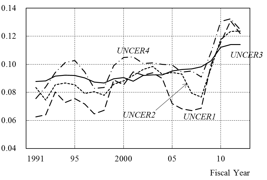Figure 1. Yearly Sample Means of the Uncertainty Measures across Firms

4. Results

4.1. Measure of Two Industrial Characteristics

To empirically examine our two hypotheses, we discuss the index used to measure the degree of competition in the products market and the degree of irreversibility of capital goods.

4.1.1. Degree of Competition in the Products Market

The degree of competition in the products market is used to examine hypothesis 1. The Herfindahl index and the k-firm concentration ratio, both indicators for the market share of products, are the most popular indices for measuring the degree of competition in a products market. Ghosal and Loungani (1996) also used a 4-firm seller-concentration ratio as a measure of market competition. However, since this index is targeted only at firms that have already achieved market entry, the viewpoint of contestability—the degree of entry barrier to a market—is missing. Given the problem produced by measuring the degree of competition by the k-firm concentration ratio, we must measure it according to the degree of new entry barrier. Industries dominated by large firms have a strong market entry barrier, while industries dominated by small firms have a lesser one. It is thus possible to capture the size of barriers to market entry by measuring the firm size for each industry.

Although domestic market competition is the ground of the above argument, the measure of market competition can also include an overseas market. However, when the degree of market competition is examined from the viewpoint used in this paper, competitive pressure from overseas is not satisfactory. One of the factors in trade breakouts, as Krugman (1980) emphasized in trade theory, is product differentiation. Since a certain monopolistic situation developed in the field where product differentiation progressed, it may be unsuitable to treat export and import size as a proxy for degree of market competition. Excess profits are also used to indirectly capture the degree of market competition. If excess profits exist under perfect competition, a new entry will occur immediately, and the excess profits will disappear. By contrast, a monopolistic profit is maintained in a monopoly situation. Therefore, the degree of market competition can be indirectly assessed from the excess profits. Based on this idea, Guiso and Parigi (1999) adopted the markup ratio as a measure of market competition.

The features of each index are taken into consideration, and two indicators were adopted as measures of market competition. One is a Herfindahl index, explaining the market share, and the other is the average size of firms, expressing the size of the barrier to market entry, which accounts for the contestability that the former lacks.

Herfindahl Index

We adopted a Herfindahl index from the JIP (Japan Industrial Productivity) database of the Research Institute of Economy, Trade and Industry. The index is constructed based on data on individual firms in the Establishment and Enterprise Census of the Statistics Bureau. Small and medium-sized enterprises other than listed companies are also included.

The index is computed using the number of employees rather than sales; the proportionality relation of the number of employees and sales is assumed. It is defined as follows:

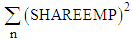(7)

where SHAREEMP: the share of the number of employees of each company within the industry,

n: the number of companies within each industry.

The manufacturing industry is classified into 52 industry types in the JIP database, the classification of which is designed to correspond to the Japan Standard Industry Classification through a converter. Since the data for 1996, 2001, and 2006 were obtained during an analysis period covered, the average for three times was adopted.

As mentioned, this index lacks contestability. The k-firm concentration ratio and Herfindahl index are the indices that should be computed for each product, and it is difficult to measure a market share correctly from the entire sales of a firm if the firm manufactures two or more products that should be considered in another product market.

Firm-size Classes

We capture the degree of market competition indirectly by measuring the size of the barrier to market entry. We measure the size of this barrier according to the average size of firms based on the number of employees for each industry. They are classified into 122 types of industry according to the classification of the Development Bank of Japan. This is not strictly the same as the Japan Standard Industry Classification because it is based on the two-digit figure grouping of the Japan Standard Industrial Classification and contains some parts of three-digit figure groups.

First, the sum total of the employees of each industry is divided by the number of firms in the industry. This calculation is repeated for each year from 1991 to 2012, and the average for 22 years is used to eliminate deflection by the abnormal value of each year.

As the computation uses data for listed companies only, not all firms that have participated in the market are included.

4.1.2. Degree of Irreversibility

Degree of irreversibility is used to examine hypothesis 2. Ogawa and Suzuki (2000) adopted the life of equipment as the irreversible index under the assumption that the secondhand market for products in Japan was vulnerable. However, as described in Section 2.2, the degree of irreversibility depends, for example, on the existence of secondhand markets for capital goods, the prices for used products, the existence of a rental market, and the possibility of diversion to other industries. This paper uses two measures of the degree of irreversibility, at the industry level rather than the firm level. These industry-level data are based on the Census of Manufactures of the Ministry of Economy, Trade and Industry for every industry. We adopt the two-digit industrial classification.

Share of Used Capital Expenditures in Total Capital Expenditures

The degree of irreversibility of capital goods depends on the existence of a secondhand market or the difficulty of accessing one. Guiso and Parigi (1999) captured the measures from interview data. Pattillo (1998) used the ratio of the real sales value of the capital stock to its real replacement value as an indicator of the irreversibility of investment, taking into consideration Ghana’s substantial secondhand market for equipment. It is difficult to construct the same index in Japan due to data restrictions. We compute the ratio of used capital expenditures to the total capital expenditures. This is the rate of the “value of second-hand assets” to the “value of tangible fixed assets excluding land” in the Census of Manufactures. Since the data for 1990, 1995, 2000, and 2005 were obtained at an analysis period covered, the average for four times was adopted. A high share implies the existence of an active secondhand market for capital in that industry. We believe that the gap in these shares among industries reflects a difference in the completeness of the secondhand market.

Rental Rate of Capital Goods

If capital goods are flexible rather than firm-specific, they may be diverted to other firms or industries, or they could be easily leased. Cassimon et al. (2002) used leasing as an indicator of access to a secondary market. We compute the rental rate of the industry’s capital goods as an indicator of the flexibility of equipment. This is the rate of the “value of lease contracts” to the “value of tangible fixed assets excluding land” in the Census of Manufactures. Since the data for 2000, 2005, and 2010 were obtained at an analysis period covered, the average for three times was adopted. A high rate indicates an active secondhand market, which implies that the capital goods are easily transferred between firms within these industries.

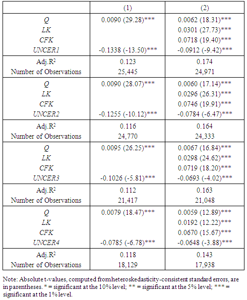
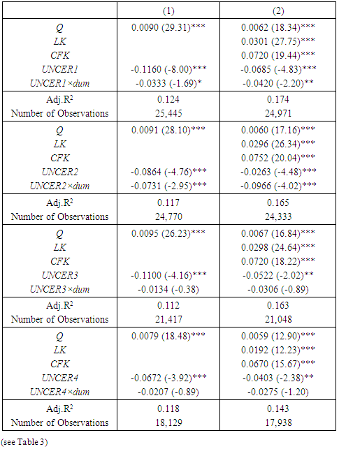
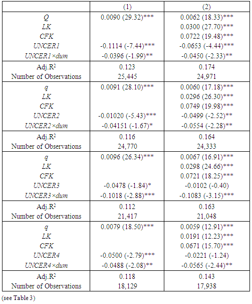
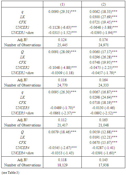
4.2. Estimation Results

We now estimate the investment function with an uncertain measure among the explanatory variables and examine the relationship between uncertainty’s effect on fixed investment and the industrial characteristics. A fixed-effect or random-effect model was discerned by the Wu-Hausman test, and a suitable estimation result is reported. The estimation period covers 1991 to 2012, as mentioned.

First, the estimation results of the basic investment function shown in Section 3.1. are displayed in Table 3. All the coefficients of q, LK, and CFK show correct and significant signs, and the effects of Tobin’s q and the role of land used as collateral and internal financing are quite satisfactory. Moreover, the effects of uncertainty on investment are altogether negative, as expected, and significant results at the 1% level are obtained. Therefore, we can conclude that the negative relationship between uncertainty and investment seems robust.

Table 3. Estimation Results of the Investment Function with the Uncertainty Measures

As seen below, we examine the two hypotheses using a dummy variable (DUM) taking unity for firms in the industries with low competition in product markets (or high irreversibility) and zero otherwise. They are constructed by a sample split at the median on the basis of the indicators shown in Section 4.1. A cross-product of the uncertainty measure with the dummy variable is added in the investment function.

Hypothesis 1

To examine hypothesis 1 (that uncertainty has more negative effects on investment in an industry with low competition in market products than in one with high competition), we construct a dummy variable by a sample split on the basis of the indicators used to measure the degree of competition in the products market and estimate the investment function adding a cross-product of the uncertainty measure with the dummy variable. The cross-product is expected to be significantly negative. The results are satisfactory, as shown in Table 4. The uncertainty measure has a negative effect on investment, and the cross-product of the uncertainty measure with the dummy variable exerts a significantly negative effect. We find a clear difference according to the degree of market concentration.

Table 4. Market Competition and the Investment–Uncertainty Relationship: Herfindahl index

When the size of market entry barriers are measured by firm-size classes, the cross-product of the uncertainty measure with the dummy variable is expected to be significantly negative. The estimated results are presented in Table 5. The cross-product has a generally negative effect.

Table 5. Market Competition and the Investment–Uncertainty Relationship: Firm-size Classes

Ghosal and Loungani (1996) used a 4-firm seller-concentration ratio as a measure of market competition, and a strong negative relationship between uncertainty and investment was observed with a high degree of competition. However, Guiso and Parigi (1999) adopted the markup ratio as a measure of market competition and found that uncertainty had more negative effects in an industry with low competition. Our estimation results using a panel data of Japanese manufacturers support the latter study. Why was the opposite result obtained? One possible factor is the measure of market competition Ghosal and Loungani (1996) adopted. Their next study, Ghosal and Loungani (2000), assumed that industries with small entry barrier are dominated by small firms. They suggested that credit constraints expand the negative effect of uncertainty on investment because small firms have more limited access to the capital market.

However, this study adopts firm size as a proxy for the degree of market competition. Our sample comprises listed companies and does not include small companies directly affected by credit constraints. Furthermore, in our investment function, we employ two explanatory variables to control for the impact of credit constraints. One concerns the role of land used as collateral, and the other concerns the role of internal financing. Our controlling for the conditions of credit constraints produced the estimation results consistent with hypothesis 1.

Hypothesis 2

To examine hypothesis 2 (that uncertainty has more negative effects on investment in an industry with high irreversibility than in one with low irreversibility), we construct a dummy variable by a sample split on the basis of the indicators used to measure the degree of irreversibility and estimate the investment function adding a cross-product of the uncertainty measure with the dummy variable. The uncertainty measure is expected to be significantly negative in industries with a low share of used capital expenditures out of total capital expenditures. The results are satisfactory, as shown in Table 6. The cross-product of the uncertainty measures with the dummy variable has a negative effect.

Table 6. Irreversibility and the Investment–Uncertainty Relationship: Share of Used Capital Expenditures in Total Capital Expenditures

When we measure the flexibility of assets by the rental rate of the industry’s capital goods, we expect the uncertainty measure to be significantly negative in industries with a low degree of this indicator. The estimated results are given in Table 7. The negative effects of the cross product are approximately significant.

Table 7. Irreversibility and the Investment–Uncertainty Relationship: Rental Rate of Capital Goods

Our estimation results support hypothesis 2 and are consistent with Pattillo (1998), Guiso and Parigi (1999), and Cassimon et al. (2002).

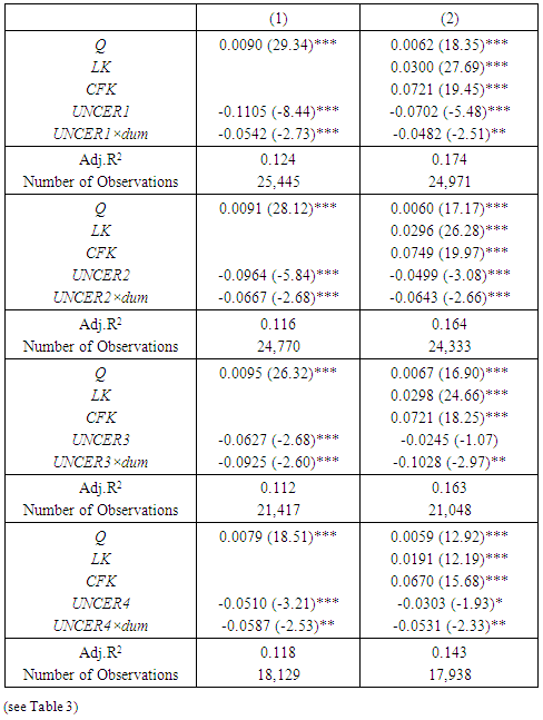
5. Conclusions

This study examines the industrial characteristics related to the strength of uncertainty’s negative effects on investment using Japanese manufacturing data. The two industrial characteristics considered are the degree of competition in the product market and the degree of irreversibility. We applied several different statistical methods to construct the uncertainty measure in order to examine the robustness of the relationship between investment and uncertainty. The uncertainty measures were constructed using each firm’s sales growth rate via the conditional standard deviation, the standard error of an autoregressive model, and the forecasting error of future prediction by an autoregressive model. The main results are summarized below.

We examined whether the degree of competition in the products market is associated with a negative uncertainty effect on investment. Uncertainty has more negative effects in industries with high market concentration and in industries with large market entry barriers. This estimation result shows that uncertainty has more negative effects on investment in an industry with low competition in the products market than in one with high competition. This suggests that the option value, the right to wait to invest, is high because the effect of the first-mover advantage is small in an industry with low market competition.

We also examined whether the degree of irreversibility of capital goods is associated with a negative uncertainty effect on investment. Uncertainty has more negative effects in industries with a low share of used capital expenditures out of total capital expenditures and in industries with a low rental rate for capital goods. When it is assumed that an investment is partially reversible, the value of a call option, the right to wait to invest, is reduced by the value of the put option, the right to wait to dispose of the capital goods. The net effect depends on the degree of irreversibility. This estimation result shows that the effect of uncertainty on investment is significantly negative for industries with more irreversible capital goods, which have low resale possibility in a secondhand market and a low chance of being diverted to other industries because the value of the put options is smaller in industries with more irreversible capital goods than in other industries.

Our findings suggest that competition in the products market mitigates a negative uncertainty effect on investment and that the irreversibility property of the investment aggravates that effect. Of course, we cannot infer from this empirical study alone a relationship between the effect of uncertainty on investment and industrial characteristics. More empirical studies are needed to examine the robustness of our results. We intend to conduct several further empirical studies. First, since we found that two industrial characteristics—competition in the products market and the irreversibility of capital goods—had effects on the negative relationship between uncertainty and investment, we should determine which one between market competition and irreversibility is more important. Next, we should improve the measurement of uncertainty, reversibility of investment, and market competition. It is also important to develop the empirical specification of the investment function. Finally, as this study used data from Japanese manufacturing industries, we should expand the sample by including non-manufacturing and unlisted firms.

6. Data Appendix

6.1. Capital Stock

Since financial statistics are based on book value, most of the data required for the estimates cannot be obtained directly from financial statistics and therefore must be constructed. The data construction of capital stock is important in the empirical study of investment behavior. In this study, the data for capital stock were constructed following Hayashi and Inoue (1991).

The basic strategy is the perpetual inventory method. The benchmark of the capital stock is that for the end of the 1977 fiscal year.

Capital goods are categorized into six sets of assets: (1) nonresidential buildings, (2) structures, (3) machinery, (4) transportation equipment, (5) instruments and tools, and (6) others. Data series are constructed for each asset by firm. Physical depreciable capital stock is computed from the following formula:

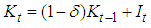(8)

where K_t: real capital stock at the end of year t,

I_t: real fixed investment in year t,

δ: physical depreciation rate.

The series for the real capital stock are calculated by totaling the real capital stock of the six asset types for each firm. Some points of argument concerning the construction process are noted below.

Nominal capital investment: The definition of nominal capital investment results from the subtraction of the book value of assets sold or retired during year t from the book value of an acquisition of assets during year t.

Price of capital goods: We use the corporate goods price index (CGPI) of the Bank of Japan to deflate nominal capital investment. The base year for the index is 2010. The price of the construction materials component of the CGPI is used for (1) non-residential buildings and (2) structures. The price index for (4) transportation equipment is the transportation equipment component of the CGPI, and, for (6) others, the manufacturing industry products are adopted. For (3) machinery and (5) instruments and tools, a weighted average of the CGPI using the weight for equipment and other capital goods in each industry given in the fixed capital matrix of the Input–Output Tables is used for the price of capital goods. Specifically, the manufacturing industry is divided into 14 industries. Machinery is further divided into four categories, and instruments and tools are divided into four categories in each industry.

Benchmark: The book value of net capital stock for the end of the 1977 fiscal year, which is the benchmark of the capital stock, is obtained from financial statistics. The book value was used as a benchmark, as in Hayashi and Inoue (1991). However, the book value had to be converted into the value of the current replacement cost basis. The numerators of this conversion for the six asset types are computed using information of the book value and the value of the current replacement cost basis of tangible assets in the National Wealth Survey of the Cabinet Office. We obtain the benchmark of capital stock by multiplying the book value of net capital stock by these numerators.

Physical depreciation rates: The physical depreciation rates are based on those reported in Hayashi and Inoue (1991). They show the rates for five categories of assets, which were derived from Hullten and Wykoff (1979, 1981). We adopt 4.7% for (1) nonresidential buildings, 5.64% for (2) structures, 9.489% for (3) machinery, 14.7% for (4) transportation equipment, and 8.838% for (5) instruments and tools and (6) others.

6.2. Tobin’s q

The Tobin’s q used in this paper is calculated as the market value of a company divided by the replacement value of the company’s asset. It is defined as follows:

(9)

where LB: book value of interest-bearing debts,

V: market value of outstanding stocks,

LAND: market value of land stock,

OTHER: inventory assets and miscellaneous assets,

P: capital investment deflator (2010 base),

K: real value of capital stock.

The market value of the company is evaluated using the stock price, and the market value of the land stock is deducted from it. Therefore, Tobin’s q can be negative when a stock price is very low.

6.3. Land Stock

The series for land stock are also computed using a perpetual inventory method. The benchmark of the land stock is the end of the 1977 fiscal year. Since the deviation between the market value and book-value of land is thought to be large, the market value of land stock as the benchmark is computed by multiplying the book value of the land stock in the financial statistics by the market-book ratio. Finally, the land stock at the market price is constructed through the following formula:

(10)

where : land price at year t,

ILAND_t: increment of land of book value in year t.

The six largest cities were used to establish an urban land price index; the land price data were obtained from the Japan Real Estate Institute.

In this method, the book value of the decrement of land is converted into the market value, with a FIFO-type assumption.

6.4. Cash Flow

The nominal cash flow is defined as the sum total of net income after taxes and depreciation. The real cash flow is calculated by deflating nominal cash flow by the output deflator for each industry.

ACKNOWLEDGEMENTS

An earlier version of this paper was presented at the 2005 spring meeting of the Japanese Economic Association at Kyoto Sangyo University, Kyoto, on June 4, 2005. I would like to thank Kazuo Ogawa, Soshichi Kinoshita, and Yosuke Takeda for helpful comments and suggestions. Any remaining errors are my own.