-
Paper Information
- Next Paper
- Previous Paper
- Paper Submission
-
Journal Information
- About This Journal
- Editorial Board
- Current Issue
- Archive
- Author Guidelines
- Contact Us
International Journal of Finance and Accounting
p-ISSN: 2168-4812 e-ISSN: 2168-4820
2016; 5(5A): 1-29
doi:10.5923/s.ijfa.201601.01

The Development of Investment Research and Multiple q in Japan*
 Abstract
 Reference
 Full-Text PDF
 Full-text HTML
Kazumi Asako1, Jun-ichi Nakamura2, Konomi Tonogi3
1Rissho University and Hitotsubashi University, Japan
2Research Institute of Capital Formation, Development Bank of Japan
3Rissho University, Japan
Correspondence to: Kazumi Asako, Rissho University and Hitotsubashi University, Japan.
| Email: |  |
Copyright © 2016 Scientific & Academic Publishing. All Rights Reserved.
This work is licensed under the Creative Commons Attribution International License (CC BY).
http://creativecommons.org/licenses/by/4.0/

Empirical deadlocks Tobin's “q theory” had confronted initiated the various lines of research which have tried to improve the empirical performance of investment function, such as better measurement of q, structural estimation, and introduction of irreversibility or fixed costs in the adjustment process. We review and argue all of these developments successfully have captured certain aspects of investment behavior that previous theories cannot. However, there is no single model that can explain every aspect of investment alone, mainly because of substantial heterogeneity in investment behavior depending on the type of capital goods or the difference between new acquisition (positive investment) and sale/retirement (negative investment). In the second half of the paper, we estimate a non-linear version of the Multiple q investment function, which can explicitly handle the aforementioned heterogeneity, on the micro data of Japanese listed firms. We confirm our non-linear model dominates the traditional linear Multiple q model and find great dispersion in the range of non-linearity depending on time and the type of capital goods.
Keywords: Capital goods heterogeneity, Lumpy investment, Multiple q, Non-linear investment function
Cite this paper: Kazumi Asako, Jun-ichi Nakamura, Konomi Tonogi, The Development of Investment Research and Multiple q in Japan*, International Journal of Finance and Accounting , Vol. 5 No. 5A, 2016, pp. 1-29. doi: 10.5923/s.ijfa.201601.01.
Article Outline
1. Introduction
- The first half of this paper is a review of the research on capital investment in Japan aiming to be a sequel of Asako and Kuninori (1989). The changes in circumstances surrounding the Japanese economy and corporate investment that have taken place in the last 25 years gives us a sense that then and today belong to completely different ages. Much of the investment implemented during the bubble economy or the latter half of the 1980s became excess capacity and firms came to suffer from having to deal with it. A number of factors combined in Japan, including the turmoil in the financial sector and the systemic fatigue in the socioeconomy as a whole that was unable to respond to the rapid globalization and to the aging population, and Japanese firms lost the momentum that they had in the past. Moreover, the situation has changed greatly not only in Japan, but throughout the world. Due to the overblown financial sector, to the rising economic power of emerging countries, and the rapid progress and spread of information and digital technologies, the importance of physical capital has decreased relatively, whether for economic growth or for corporate management, and instead the focus is now being placed on the role of intangible assets, such as human capital and brand value. Nevertheless, it is certainly not the case that researchers’ interest in investment has waned recently. That the empirical performance of “q theory,” which was regarded as a refined investment theory based upon the micro foundations of the neo-classical school to the ideas of Tobin (1969), had been disappointing was basically the consensus among researchers at the time of writing of Asako and Kuninori (1989). This “puzzle” stimulated the motivation of researchers and they searched in a range of new research directions, either to modify or to supplement q theory. In terms of modifying theories, in place of the convex adjustment costs that q theory assumed (namely, investment behavior with short and quick adjustments with regards to changes to expected earnings), the “lumpy and intermittent/infrequent investment” model was proposed that explained behavior through the existence of a fixed-costs part in adjustment costs and investment irreversibility. The fit of this kind of model with reality is supported by individual data at the level of plants or establishments, and currently it has established a position as one of the standard analytical frameworks. However, the objective of this paper’s review, the same as in Asako and Kuninori (1989), is not to provide a comprehensive overview of the accumulation of this enormous body of research. A detailed overview of the developments in investment research in recent years have already been provided by, for example, Caballero (1999), Hayashi (2000), and Bond and Van Reenen (2007), and moreover, in the Japanese literature, by Suzuki (2001) and Miyagawa (2005). Rather, what we emphasize in this paper is the following point taken from the findings of the new research developed since the second half of the 1980s; that the clarification of two types of heterogeneity―namely, differences in investment behavior according to capital goods, and differences in behavior to new acquisition of capital goods (positive investment) and to sales and retirements of those (negative investment)―have emerged as being one of the major problems remaining for empirical research. Capital stock that firms actually possess is composed of many classifications of capital goods, such as buildings and machinery. Different investment patterns are seen for each classification of capital good has been well known for a long time, such as the building cycle (or Kuznets swing) and the cycle of investment in machines (or Juglar cycle). However, in almost all cases, the standard investment models and empirical studies, as represented by q theory, assume that the abstract concept of homogeneous capital stock is the only quasi fixed factor or that in short all capital goods are homogeneous. Moreover, with regards to differences in inflows (positive investments) or outflows (negative investments), a gross flow analysis in which job creation and job destruction are not cancelled each other and treated separately came to be commonly used from an early stage in employment analysis, but its feature has been almost entirely neglected in investment analysis.It can be said that the main reason why such a simplification has continued even with the poor performance of empirical analyses is data constraints. Paradoxically, the increasing use of data on the level of plants and establishments that has occurred within the trend toward giving importance to micro data in recent years has in some respects spurred this problem. For example, in the case of listed firms in Japan, detailed statements of tangible fixed assets according to capital goods are disclosed at the firm level, but not at the level of plants and establishments.1 In addition, with regards to the gross flow of investment, a problem is that when negative investment takes the form of the abolition of plants and establishments, this becomes missing data at the micro level.2In the second half of this paper, detailed data on the tangible fixed assets of Japanese listed firms that has been accumulated over many years by the Development Bank of Japan is used, and an empirical analysis is performed based on “Multiple q model” which is a modified version of the standard q model of investment to deal with the heterogeneity of multiple capital goods. Theoretically, the Multiple q model was first proposed by Wildasin (1984) and then applied to empirical analyses by Asako, Kuninori, Inoue, and Murase (1989, 1997). Based on this previous research, our empirical Multiple q model is generalized further to be able to deal with differences in positive or negative investment behavior and to include cases where the convex adjustment cost that is a prerequisite of the q model is not necessarily appropriate. After the abnormal upsurge in investment in land and buildings in the bubble-economy period, Japanese firms went through a process of excess capacity reduction (negative investment) after the bubble collapsed. We exploit the development as a good source of data in order to analyze heterogeneity from classifications of capital goods and positive or negative investment. And at the same time, the results of this analysis go beyond simply being of academic interest and could be an important basic material when considering the revival of Japanese firms. The rest of this paper is organized as follows. In Section 2, first we review the various attempts of previous studies to improve empirical performance within the framework of the q theory. In addition, based on its limitations, we provide an overview of the directions taken to theoretically augment it that are supported by observations of micro data. In Section 3, after arranging the various augmented models discussed in Section 2 under a unified view of the differences in the formulation of the adjustment cost function, we review the results of the empirical analyses that have used the augmented framework. From Section 4 onwards, we introduce our attempt to explicitly incorporate into the analysis the two types of heterogeneity that represent one of the major remaining problems for empirical analysis, of differences in capital goods and differences in positive or negative investment behavior. In Section 4, we first explain the augmentation of the Multiple q investment function to include nonlinear cases, and also the method of empirical analysis. In Section 5, we report the main estimation results and consider their implications, and in Section 6 we provide a concluding summary and remaining issues for future work.
2. The Research Development of Post q Theory
2.1. The q Theory and the Failure of Empirical Research
- In this investment theory, which has been called Tobin’s q theory ever since it was proposed by Tobin (1969), q is defined as the ratio obtained by dividing the firm’s market value―in other words, the cost of purchasing the firm in its entirety―by the total cost of replacing the capital stock held by that firm. If q >1, then capital investment is being carried out. This ratio is a value that is actually observable in the data, called “average q”. However, as is generally known, this proposition is nothing more than a claim that real investment is more advantageous than holding shares and does not decide the flow volume of investment. If based on the microeconomic foundations of neo-classical firm theory, marginal q should be used, which is the ratio of the marginal increment of firm value resulting from the implementation of one unit of investment (the imputed price of capital), and the replacement cost of the marginal capital stock (the market price of capital goods). Actually, as a trend separate to Tobin (1969), by taking into consideration the adjustment cost of investment, determining flow investment at the point where an investment’s total marginal cost (the sum of the market price of capital goods and the marginal adjustment cost of investment) is equal to the imputed price of the capital becomes the optimal behavior for a competitive firm, as is already known from research such as Lucas (1967), Gould (1968), and Uzawa (1969). As an extension to this, an investment function in which the flow volume of investment corresponds to marginal q on one-to-one basis as the results of firms’ dynamic optimization behavior was derived by Lucas and Prescott (1971), Mussa (1977), Nickell (1978), and Abel (1980). Further, Yoshikawa (1980) and Hayashi (1982) showed the condition for average q to become equal to marginal q,3 and when estimating with the investment function, they provided a theoretical rationale for the use of average q instead of marginal q, which is difficult to observe directly. In this way, neoclassical micro foundations were added to Tobin’s ideas to complete the “q theory.” This q theory, as indicated by Asako and Kuninori (1989), included special cases, such as the acceleration principle that has been used from long ago as a capital stock adjustment theory, and the so-called Jorgensen model based on the concept of the user cost of capital, and it was appealing as a “unified theory”. Moreover, q theory was expected to become a powerful analytical tool for empirical researchers. Specifically, based on q theory, the conclusion is reached that the same as marginal q, average q becomes a sufficient statistic for investment volume, and consequently variables other than q become redundant with no additional explanatory power. Further, if we allow the adjustment cost function to be formulated approximately with the quadratic function of investment ratio, it is possible to obtain an investment function that is extremely simple and also easy to estimate, in which the investment ratio is obtained as a linear function of average q only. However, in contrast to the theoretical conjecture, the explanatory power with regards to actual investment data from estimates of the linear investment function using average q was proved to be unsatisfactory and perceived to be a problem from the beginning.4 The following features arranged by Asako and Kuninori (1989) summarize its problems. (1) The explanatory power of q, which should be a sufficient statistic of the investment rate, is not all that high (the q coefficient is not significant, or even if it is significant, the coefficient is extremely small).5(2) When variables other than q are added to the list of explanatory variables, such as cash flow, value of output, and capacity utilization ratio, these variables become significant and in some instances, decrease the explanatory power of q itself.6(3) A major serial correlation is seen with the residual term, and past q’s become significant as an explanatory variable.Since the second half of the 1980s, a main problem in investment function research has been either investigating the cause of these problems or trying to solve them, and various directions have been attempted. If we arrange these attempts roughly, regardless of time ordering, they might be arranged into the following four categories; (i) the search for a better q, (ii) re-examinations of the estimation equation, (iii) the appearance of new theories, and related to this, (iv) the deep plowing of micro data. The findings of each are summarized below.
2.2. The Search for a Better q
- In this direction, earlier studies aimed to improve average q itself, which includes research into tax-adjusted q that explicitly considers the effects of the tax system on firm value and investment cost, such as corporate income tax, investment tax credits, and the corporate tax saving effects of depreciation and amortization expenses. In the United States in the 1980s, the investment environment changed greatly following the introduction of and the amendment to the Reagan tax system. Being motivated by the fact that the measurement of policy effects had become a hot issue, empirical studies of the investment function using tax-adjusted q were actively conducted. Tax-adjusted q to a certain extent played a role in improving the performance of estimates of the investment function during a period when the tax system greatly changed, but it did not provide a far reaching solution to the problems of average q. It was also limited on the point of considering the effects of the tax system, as for example, it unavoidably hypothesized static expectations on the future tax system.On the other hand, an even bigger question was raised that there might be a more fundamental problem for the use of average q instead of marginal q. As a result, an idea gained credence that it might be more productive to investigate a method of estimating marginal q from other observable variables (below, this is called the marginal q approach). One of the fundamental problems was that the theoretical assumptions used to justify average q―namely, the production function’s and adjustment cost function’s first order homogeneity and perfect competition in the product market―had not been established. Another problem was it was possible that there was a distortion that would be impossible to ignore for stock prices that are indispensable for the measurement of firm value, which is the numerator of average q.7However, with the starting point being that marginal q cannot be directly observed, and therefore the use of average q became common place, we should incur some cost in order to obtain the estimation value of marginal q. That is to say, entrepreneurs’ expectations for capital's marginal revenue and discount rate over an unlimited period in the future have to be specified and a strong assumption has to be made for this part. Typically, it is assumed that the stochastic process that generates the profit rate and discount rate in the future is stable, and entrepreneurs’ expectations are estimated using the VAR (vector autoregression) model based on past actual values. This method introduced by Abel and Blanchard (1986) and Otaki and Suzuki (1986) has been widely used.8For example, Ogawa and Kitasaka (1995) used this method and calculated marginal q according to industry in Japan from 1970 to 1990, and compared the results to average q. They considered that if marginal q is appropriately measured, the deviation of average q from marginal q will reflect monopolistic rent based on imperfect competition or a stock-price bubble. With a result of this analysis suggesting that the deviation of average q from marginal q is non-stationary and that this deviation is not completely explained by monopolistic rent, they concluded that average q contains bubble and fads elements. Further, Ogawa and Kitasaka (1998) compared the empirical performance of investment function utilizing average q from data according to industry in Japan during the same period with investment function utilizing marginal q, and found the latter to be the winner.9 However, even in the results of their estimates of the investment function by marginal q, the q coefficient itself was small, but in contrast, the explanatory power of cash flow and land assets was high. So it was not the case that the problems facing the use of average q for the investment function has been fully conquered. We can also find plenty of examples of marginal q becoming significant by incorporating liquidity constraints among foreign studies though, as summarized by Whited (1998), it cannot be said that there has been any drastic improvements in overall empirical performance and in resolving the problems when compared to average q.
2.3. Re-examinations of the Estimation Equation
- Regardless of the various efforts to improve q, if we simply accept the fact that cash flow has strong explanatory power for investment, it is natural to interpret it as evidence that imperfections in the capital markets, such as liquidity constraints, have some sort of effect on investment. Therefore, keeping in mind the credit crunch in the United States at the beginning of the 1990s, and as a case in stark contrast to it, the relations between firms and banks in Japan, there has been a rapid development of research that has attempted to investigate the effects of capital market imperfection using investment-cash flow sensitivity as an indicator.10 However, this method is susceptible to various problems due to the estimation of the investment function based on q theory; for example, it is easily influenced by issues such as the measurement error of q and the simultaneous equation identification problem, and moreover, the failure to establish the preconditions of q theory (for example, perfect competition). Therefore, it has been subject to a lot of criticism that investment-cash flow sensitivity might capture something different from the imperfection of the capital market. But at the same time, this criticism has resulted in increasing opportunities to re-examine a better estimation equation for the investment function.First to be examined was the problem of simultaneity. That is to say, because q and investment are both decided simultaneously as endogenous variables, it is possible that this generates bias in the OLS (ordinary least squares) estimator, which in turn generates the spurious explanatory power of cash flow. Actually, Hayashi and Inoue (1991) showed that if the simultaneity problem was controlled by adopting the instrumental variable method, the significance of cash flow declined. However, the estimate of the q coefficient, even significant, remained as before a small value.Moreover, not limited to cash flow, it must be said that the ad-hoc adding of variables other than q to the list of explanatory variables for the investment function lacks theoretical foundations. With regards to this, Hubbard and Kashyap (1992) and Whited (1992) added a borrowing constraint to the optimization problem of q theory, and assuming that the undetermined multiplier pertaining to the borrowing constraint is a function of variables such as land assets and future earnings, estimated the Euler equation and, attempted to verify the imperfection of the capital market with a certain theoretical foundation. Among the first-order conditions of the dynamic optimization problem concerning investment, the Euler equation expresses the dynamic conditions that the imputed price of capital must satisfy over time. Substituting out from this expression the imputed price or the marginal q term by making use of the first-order condition (the q equation) that gives the relationship between investment and q, one can estimate the resultant investment function. This idea (the Euler equation approach) has existed since Abel (1980), but it can be said that it came to be widely used as a result of the debate on the imperfection of the capital market. The greatest benefit of this approach for empirical research is that the value of q is not required for estimation of the investment function. In other words, not only is it not necessary to assume perfect competition and an efficient stock market in order to justify using average q instead of marginal q, it is also not necessary to make additional assumptions regarding the process of forming expectations for estimates of marginal q, and consequently it is free from the measuring-error problem.11However, it is difficult to say that this Euler equation approach has achieved sufficient success in a practical sense. Specifically, as was pointed out by Whited (1998), in many cases the over-identification constraint test of GMM (Generalization Moment Method), which is the typical estimation method, is cleared, and this suggests the possibility of a misspecification in the formulation. Also, Oliner, Rudebusch and Sichel (1995), who used aggregate data according to capital goods in the United States, carried out a competitive comparison of predicted performances of various investment models and found that the Euler equation approach was inferior to traditional models, like the acceleration principle, and the q model. Further, Oliner, Rudebusch and Sichel (1996) pointed out that, from the perspective of the criticism of Lucas, the estimation value of the structural parameter from the Euler equation that ought to be stable is in fact, unstable. The same as with the marginal q approach, we can find various other studies that show an improvement to explanatory power through imposing a constraint of capital market imperfection. But even if their results are robust, it seems reasonable to consider that they have only succeeded in eliminating just a small part of the problems q theory faces.
2.4. The Appearance of New Theories
- As was described above, attempts to improve q theory in the shape of maintaining the fundamental framework of it have run up against a brick wall. In this context, the validity of the convex adjustment cost (investment behavior that makes short and quick adjustments with regards to changes to expected earnings), which is an indispensable precondition of q theory, began to be questioned from its foundations, and research aiming to build a new theory gradually began to increase; specifically, a model of lumpy and intermittent/infrequent investment behavior that explained through the existence of a fixed-costs part in the adjustment cost and investment irreversibility.If we assume that the optimal capital stock level given expected earnings is uniquely decided, a gap with the optimal level is generated by an exogenous change to expected earnings. At this time, if adjustment costs do not exist, the gap should always be instantaneously adjusted and the flow investment volume will not be decided. Therefore, as the mechanism that decides the investment volume, in q theory convex adjustment costs are built into the model. Under the convex adjustment costs (typically, the quadratic function of the adjustment volume or the adjustment rate), as the adjustment width grows, the additional adjustment costs gradually increase. Consequently, when the newly generated gap is large, it is not optimal to fill all the gap at once. Instead, it is optimal to take a sort of “leveling” action which adjusts the left-over part when the new gap is small. However, in this sort of smooth adjustment process, there is a contradictory aspect of the well-known severity of the fluctuations of investment in the context of business cycles. Lumpy and intermittent/infrequent investment indicates investment behavior in during a period when investment is not done at all (inaction) continues for a while and then a large-scale investment is made all at once. To say this in another way, even if capital stock diverges somewhat from the optimal level, it does not immediately bring about behavior, and when the gap exceeds the threshold value, the adjustment is done all at once (the so-called (S,s) policy or bang bang policy). As is also clear intuitively, a typical case when this sort of behavior is rational is a situation when fixed costs will be incurred in each round of adjustment (the higher the fixed costs, the higher the threshold value of the gap that starts the adjustment). More generally, if the technology for the adjustment shows increasing returns (the adjustment cost function is non-convex), it is known that this leads to (S,s) type adjustment behavior.On the other hand, a model that considers the influence of investment irreversibility has attracted attention as another mechanism for selecting inaction or zero investment despite capital stock deviating from the optimal level. Investment irreversibility is a property of capital stock that once installed, is difficult to convert to other purposes and that once the investment is done, it cannot be undone. The importance of this property had previously been pointed to by Arrow (1968), but it once again became the focus of attention from the second half of the 1980s, when the movement searching for an alternative to q theory became active, from the perspective of analyzing the suppressing effect that uncertainty has on investment. As a result, a body of research on it had been accumulated by the first half of the 1990s.12 Typically, investment opportunities resulting in uncertain investment earnings with defined costs are assumed to be (i) completely irreversible (the investment amount completely becomes a sunk cost, or the amount recovered from a negative investment is zero) and (ii) exclusive (there are no concerns that the investment opportunity will be stolen by rival firms, even if it is postponed). Therefore, the possession of such an investment opportunity can be interpreted as a call option, sometimes called a real option in contrast to an option agreement, without an expiration date that can be exercised at a time that will be most advantageous for investment earnings. In this case, the hurdle (the threshold value of q) in order to execute the investment becomes higher than the case of reversible investment by the amount of the additional cost (opportunity cost) from giving up the option. So as the uncertainty becomes greater, the value of the call option rises, and the probability increases that the firm will hold back from executing the investment.However, the phenomenon of a firm whose capital stock has diverged from the optimal level but holds back from adjustment behavior (selecting inaction or zero investment) can be explained only by investment irreversibility, regardless of the presence or absence of uncertainty. Moreover, even with regards to irreversibility, it is not necessary to assume complete irreversibility as described above and it is sufficient if the sales value of capital goods is smaller than their purchase value (partially irreversible or costly reversibility), or the convex adjustment cost has an asymmetrical property in the form of a kink (that is, has a different left and right side derivatives) at the point of zero investment rate. However, as we will see in the next section, in the model of investment irreversibility or asymmetrical adjustment costs that does not include the fixed-costs part, a discontinuous part does not exist in the relation between investment and q, and therefore lumpy adjustment behavior does not appear. Abel and Eberly (1994) considered an investment model under uncertainty which incorporates partial irreversibility and a fixed cost part into traditional convex adjustment costs, and showed that investment became a monotonically non-decreasing function of marginal q with an area of zero investment in the middle. In other words, two threshold values of
 and
and  exist in q, and so
  for a positive investment,
  for a zero investment, and
  for a negative investment become the optimal. If
  , then consequently negative investment (complete irreversibility) is not observed.13 Further, in the instant that q exceeds the threshold value, the investment rate jumps from zero to the “original level” suggested by the model of convex adjustment costs without a fixed cost and irreversibility, which also explains a sort of lumpy adjustment behavior. Therefore, as they indicated in the title of their paper, Abel and Eberly (1994) claimed to have succeeded in “unifying” q theory with the fixed costs and irreversibility model. However, this claim has been criticized. Caballero and Leahy (1996) and Caballero (1999) pointed out the following. (i) The Abel and Eberly model’s fixed costs are “flow fixed costs” dependent on the length of the adjustment period and are a false analogy to the definition of fixed costs in (S,s) type adjustment behavior (say “stock fixed costs” that are not dependent on time). (ii) If considering flow fixed costs, their “augmented adjustment cost function” as a whole preserves its convex nature in which the q theory framework maintains effectiveness, but upon introducing stock fixed costs, this convex nature is lost and the monotonicity of investment function with regard to q does not hold. (iii) To explain adjustment behavior with stock fixed costs, ultimately a framework that goes beyond q theory is required. While the differences in the definition of fixed costs and lumpiness is theoretically an important topic of discussion, in the world of empirical analysis which assumes a discrete time model, identifying such differences is difficult. Therefore, in the discussion below, the definitions of “fixed costs” and “lumpiness” we have in mind are those of Abel and Eberly (1994).14
2.5. Deep Plowing of Micro Data
- These theoretical developments concerning lumpy and intermittent/infrequent investment behavior are in themselves deeply interesting, but in the process of being recognized as a framework with rich empirical relevance, the preparation and publication of individual data at the level of the plants and establishments has played a major role. From the second half of the 1980s to the 1990s, as represented by the Longitudinal Research Database (LRD) of the United States Census Bureau, original data of public statistics at the level of the plants and establishments, which previously could only be used in a totaled form, had been arranged and released as longitudinal data for research purposes. The longitudinal data up to that point had only been provided on the level of firms (and usually listed firms), so this development became a major breakthrough for empirical researchers and resulted in a lot of research taking place over a wide range of fields, such as employment and production, that utilized the characteristics of data on individual plants and establishments. If we look at capital investment at the plants and establishments level, we see there appeared a series of research studies that showed the widespread existence of lumpy and intermittent/infrequent investment behavior. For instance, Doms and Dunne (1998), which can be said to be a one of the seminal works, found many cases that showed circumstantial evidence of lumpy and intermittent/infrequent investment behavior. For example, from individual data collected in LRD on manufacturing plants and establishments in the United States between 1972 and 1988, more than half of them had experienced a large-scale investment (investment spike) of a capital stock growth rate of 37% or more in one year. Within the 16 years, there were many consecutive cases of a two year period with the largest rates of capital growth and a major part of the fluctuations in total investment volume for the sample as a whole was explained by the occurrence rate of investment spike. While weakened as the level of aggregation in the sequence of plants and establishments → business division→ firm, even at the level of the firm, to a certain extent, the property of lumpy and intermittent behavior still remained. Moreover, in a comparison at the plants and establishments level, they found that the smaller the scale of the plants and establishments, the more pronounced the lumpiness and intermittentness, and they thought that this suggested the indivisibility of capital.In addition, as a development in empirical research that advanced a step forward from simple observations of data, Caballero, Engel, and Haltiwanger (1995) focused on the “distribution” of the gaps between the optimal level of capital stock at each plants and establishments and their actual levels in order to clarify the relationship between micro-level lumpiness and intermittentness and macro-level changes to investment. In addition, Caballero and Engel (1999) modeled this idea into a more formal manner and verified the existence of lumpiness and intermittentness through the investment function totaled on the level of industries.15 As another research development, Cooper, Haltiwanger, and Power (1999), based on lumpy and intermittent/infrequent investment behavior, theoretically showed that the probability of occurrence of investment spike increased in conjunction with the length of time that has lapsed since the last spike, and this finding was supported by micro data.16
3. The Point Reached by Investment Research and the Heterogeneity of Capital Goods
3.1. A Comparison of Models using a Comprehensive Adjustment Cost Function
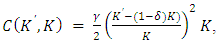
- As described in the overview in the preceding section, starting with the dissatisfaction with the empirical performance of q theory, a new theoretical framework was developed, and utilizing the opportunity provided by access to data on the level of plants and establishments, investment research in general made major progress both theoretically and empirically from the second half of the 1980s through to the first half of the 2000s. Building on this progress, Cooper and Haltiwanger (2006) considered a comprehensive adjustment cost function that encompassed q theory and a new theoretical framework and tried to compare each theory through estimating their parameters. This research provides a benchmark to confirm the point attained by investment research and its remaining problems. Below, the main points under discussion will be reconfirmed while referring to the framework of this paper.Firms’ owner managers, after observing the management environment (say productivity shock
 ) at the start of each period, solve the problem of dynamic optimization in order to maximize firm value, which is net cash flow’s present discounted value up to the infinite future, and make investment decisions. Apart from capital depreciation and the adjustment costs of investment, firms’ gross profit function is assumed to be
 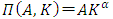 , where the parameter
  expresses technological characteristics or market power, and if
  , it is consistent with the assumptions of standard q theory of perfect competition and constant returns to scale. Furthermore, let the replacement cost of capital goods be p and capital accumulates according to
 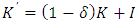 , where
  denotes capital stock at the beginning of the next period (or the end of the current period), K capital stock at the beginning of the current period,
  the capital depreciation rate, and I the capital investment in the current period. In other words, it is assumed that investment in the current period does not contribute immediately to production in the current period (it contributes to production from the following period).17 Below, as long as not particularly mentioned otherwise, when a negative investment is carried out, the sales value is equal to p, while the cash outflow from a capital investment (the purchase of capital goods) and the cash inflow from a negative investment are both expressed by
 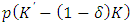 . Under the above-described assumptions, when the maximization problem for firm value V is solved using dynamic programming, and when
  is the discount factor and
  the expected value operator based on the forecast productivity shock in the next period based on current period information, the Bellman equation for optimality becomes as follows:
  | (1) |
 with regards to the investment rate
 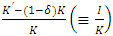 is introduced, and the Bellman equation can be rewritten as
  | (2) |
 then we have
 (2′)Here, from the first-order condition with regards to K’ or
  (the subscript expresses the partial derivative), we obtain the investment rate function
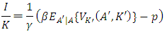 | (3) |
 is the marginal increment of firm value expected at the beginning of the next period by adding one unit of capital―in other words, the imputed price of capital―and
  is Tobin's marginal q as it is the ratio of the current value discounted imputed price of capital
  and the replacement cost of capital p. When equation (3) is rewritten by explicitly introducing q, it becomes
 (3′)and a familiar investment function that becomes linear for q is obtained.18Further, if
  , the value function V becomes linear homogeneous with regards to K, and therefore
 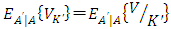 is established, and marginal
  in equation (3') can be rewritten in the exact sense by average
  . This framework is called “Model 2”. On the other hand, in order to explain lumpy and intermittent/infrequent investment, it is necessary to introduce non-convex adjustment costs which incorporated the fixed-costs part with regards to the investment rate
  or to assume investment irreversibility. It should be reminded, however, as was pointed out in Section 2.4, that lumpiness does not follow from the investment irreversibility alone.If non-convex adjustment costs are introduced, the Bellman equation can be written as follows:
  where, for
  .
. | (4) |
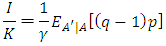
 when a firm selects zero investment (inaction) and firm value
  when a firm selects either positive or negative investment (action), the larger of the two will be selected. When zero investment is selected, there are no changes to cash flow resulting from the purchase or sale of capital goods and adjustment costs. On the other hand, when either positive or negative investment is selected, it is assumed that typically two classifications of fixed costs will be generated. The first of these is an opportunity cost type which assumes that operations are suspended temporarily due to the implementation investment (
 corresponds to the ratio of suspended period). For this type of fixed cost, if
  is a constant, the better the business conditions (productivity A is high) the stronger it works as a suppressing factor of investment (say, Model 3). The second is a capital proportionate type of fixed costs, FK, in proportion to the scale of the capital stock K (say, Model 4). Finally, when assuming investment irreversibility as Model 5, generally it is incorporated into the model in the form of capital goods’ sales value
  falling below their purchase value
  . For example, we can consider the following Bellman equation:
  where
where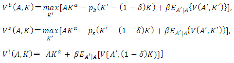 | (5) |
 .What Cooper and Haltiwanger (2006) did was essentially a competitive comparison of the empirical performances of the above five models, from Model 1 to Model 5 (no adjustment costs, convex adjustment costs, non-convex adjustment costs incorporating opportunity cost-type fixed costs, non-convex adjustment costs incorporating only capital proportionate fixed costs, and investment irreversibility), and rather than estimating the corresponding investment function, used the following method.That is to say, as the first step, based on the data of investment at the plants and establishments level collected in LRD described in Section 2.5, four statistics were chosen as the statistics thought to best represent the features of the data set; the occurrence rate of each positive or negative investment spike (the absolute value of investment rate is 20% or more); the serial correlation of investment; and correlation between productivity shock and investment. For each of the above described models, a competitive comparison was carried out through a simulation to determine to what extent they could reproduce the four statistics. As a result, while it was found that the models fit with one part of the statistics―namely, the non-convex adjustment cost (Model 3, Model 4) with the occurrence rate of a positive investment spike, and investment irreversibility (Model 5) with the occurrence rate of a negative investment spike and the serial correlation of investment―it was confirmed that none of the models was able to sufficiently explain all of the statistics independently. Therefore, as the second step from the same LRD data set, by estimating by SMM (Simulated Method of Moment) the parameter
  of the Bellman equation that encompasses all of these models (excluding Model 1 of no adjustment costs) and maximizes the following firm value V,19
 where
where | (6) |
 .With regards to the four statistics (moment) used in the first step, SMM is used to select the parameter value that will result in the smallest divergence between the actual data and the simulated moment. Therefore, it is evident that the fit will improve compared to the first step, but what is important was that all parameters were estimated significantly and that they confirmed the fit worsened if any of the single models are excluded. In other words, by combining the various types of models that have been proposed since q theory, finally it became possible to secure explanatory power commensurate to the actual data.20 According to Cooper and Haltiwanger (2006), this reflects the fact that the different adjustment processes are adopted for different types of capital. Hence, they pointed out that as long as data for each capital goods could not be obtained, the hybrid type model would be effective.
 3.2. Estimation of Non-linear Investment Function and the Heterogeneity of Capital Goods and Positive or Negative Investment
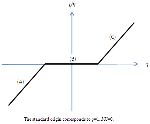
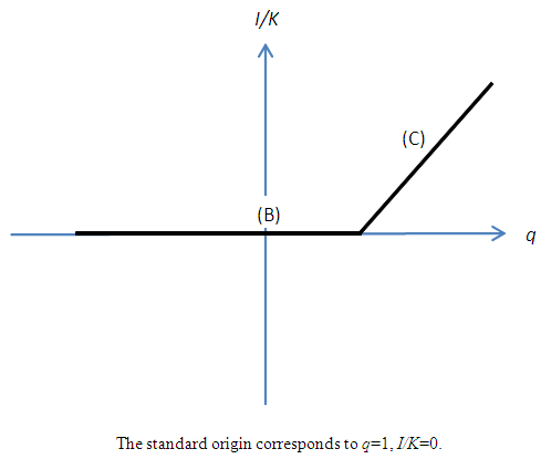
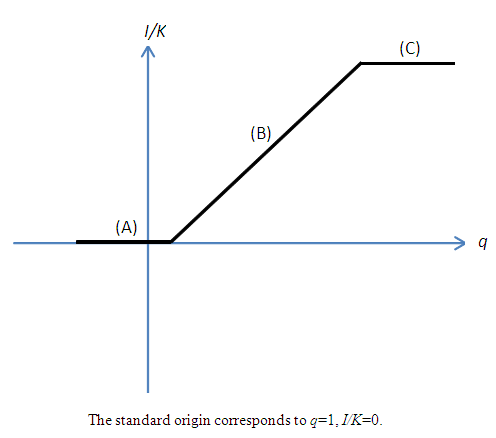
- Due to the increasing complexity of investment theories and the spread of structural estimations, empirical research aiming to explicitly estimate the investment function is not being carried out as actively as before. However, it is not the case that it has lost its importance as an analytical tool that enables an intuitive argument. If fixed adjustment costs and investment irreversibility exist, theoretically investment behavior will be unresponsive to changes to the earnings environment within a constant range. This has been also empirically supported by analyses of micro data and accepted as a new “stylized fact.” For instance, when assuming a combination of investment irreversibility (or the asymmetry of adjustment costs) and a quadratic adjustment cost function, it signifies that the relation between investment and q is not the linear investment function derived from q theory (Figure 1), but as shown in Figure 2, an N-shaped non-linear investment function that has a non-responsive part in the region around q = 1.21 While Figure 2 is drawn supposing a point-symmetry shape with regards to the origin, the slope for each of (A) and (C), and the position and width of the area of (B), depend on and can be changed by the adjustment cost parameters. For example, as an extreme case, if we assume the sales value is zero in a negative investment, the slope of (A) becomes zero and is absorbed in (B), as is shown in Figure 2′. In such estimation of non-linear investment function, the formulation of adjustment costs by Barnett and Sakellaris (1998) that simplified the model of Abel and Eberly (1994) is widely known for its convenience and has been frequently used for empirical analysis. The framework is described in Suzuki (2001) and Suzuki and Honda (2014), so we will not repeat it here. Rather, in relation to the discussion from the next section onwards, what is important is that the empirical findings on the concrete shape of this non-linearity are not necessarily consistent. Much empirical research, including Barnett and Sakellaris (1998) and Honda and Suzuki (2000), has observed an S-shaped investment function similar to a logistic curve showing the existence of a non-response part with regards to q at both ends of the distribution of q,22 as is shown in Figure 3. This can be considered to show the removal of part (A) from the non-linear investment function based on investment irreversibility suggested in Figure 2, and the addition of part (C).Regarding this, while a debate remains about whether the non-existence of part (A) in Figure 2 can be considered evidence of complete irreversibility, like in Figure 2´, or nothing more than the lack of negative investment data23, it does not contradict investment irreversibility. On one hand, the concave part with regards to q, such as (B) from (C), requires an explanation that goes beyond the framework of investment irreversibility. For example, from a theoretical perspective, one possibility is that it points to the existence of prohibitive adjustment costs with regards to an enormous investment. On the other hand, from an empirical perspective, it is considered that if average q as the proxy variable of q is used, the cause is that stock prices are influenced by a bubble economy as in Bond and Cummins (2000). If the dispersion of average q to the upper side is indeed large, then the slope of the investment function becomes flat. However, an S-shaped investment function has been widely observed even in research that did not use average q.The problem is, as in Eberly (1997) who estimated a model that encompassed several types of adjustment cost function, there have been observations of an investment function made up of only the convex part; namely, of investment that becomes more responsive to q in a higher q area.24 Against the backdrop of the mixing of the convex part and concave part with regards to q, Abel and Eberly (2002) considered the heterogeneity of capital goods. That is to say, upon allowing different threshold values of q for the upper limits of the non-responsive areas for different classifications of capital goods, while a rise of q in the area where q is low, in addition to the intensive margin that increases the investment of capital goods that have already responded to q, it results in an extensive margin that starts a response to q for capital goods that up to that time have been non-responsive,25 a rise of q in the area where q is sufficiently high results in only the intensive margin because all capital goods exceed the threshold value. At this time, if the distribution of the threshold value obeys a normal distribution, the aggregated investment function with regards to q will show an S-shape that is convex where q is low and concave where q is high.26 Eberly (1997) considered the reason why she observed the convex part in her own data while Barnett and Sakellaris (1998) observed the concave part is that the former is the balanced panel of listed firms and the latter is the non-balanced panel, including of small and medium sized young firms, and that in many cases the data of the latter corresponds to an area where q is relatively high.
3.3. Estimation of Investment Function according to Capital Good
- There has been an awareness since at the latest of Wildasin (1984), who extended q theory to cases of multiple goods, of the importance of explicitly analyzing the heterogeneity of capital goods. Today, when trends in new research that have tried to overcome the limitations of q theory in the world of single capital goods have brought about certain level of results, it is extremely interesting that once again there has come to be an awareness of the diversity of capital goods. In fact, even during the interim period, while sporadic, there was also some empirical research that focused on the heterogeneity of capital goods. Here, we will introduce some examples of research other than Multiple q that will be described from the next section. Chirinko (1993) used data on the level of firms in the United States and attempted to verify whether the poor empirical performance of the conventional q model that assumes a single capital goods was due to a misspecification of the homogeneity of capital goods or was due to measurement errors of q. First he ran the regressions of the standard q model for the macro data of structures and equipments separately and found that residual terms show serial correlation and its degree was larger for structures. Next, he explicitly considered the heterogeneity of capital goods, slightly differently from Wildasin (1984), with regards to the parameters of adjustment costs, rejected the null hypothesis of ‘capital goods are homogeneous,’ and obtained the finding that for the parameters that show the size of the adjustment costs, for structures are higher than for machinery and equipment. On the other hand, the measurement error hypothesis was rejected. Similarly, after a series of empirical research in the United States using macro data including the q model, Oliner, Rudebusch, and Sichel (1995) confirmed that the precision of estimates and forecasts for structures was inferior to those for machinery and equipment, and indicated that the reason may be that structures are composed of more diverse contents.As a reason for the low explanatory power of the q model, Goolsbee and Gross (1997) pointed out that the heterogeneity of capital was an important problem although it was not discussed very frequently. For example, when a firm buys a certain type of capital and sells a different type of capital with the same value, as long as the heterogeneity of capital is not recognized, the balance of the investment amount is considered to be zero. However, adjustments costs are not zero. Therefore they used a unique data set that captured changes to different capital goods in 16 classifications in the airline industry in the United States, and measured the shape of the investment function.27 The result suggests an N-shaped investment function like Figure 2, and the non-responsive area was clearly longer in a positive direction (on average, actions of positive investment were taken if productive capacity became 40% less than the optimal level while actions of negative investment were taken if productive capacity became 10% more than the optimal level).28 In addition, whether positive or negative, the investment function was linear in the area in which the actions were taken, suggesting the validity of standard quadratic adjustment cost function. Further, the abovementioned nonlinearity disappeared when estimating the investment function in a standard q model setting with an aggregation of heterogeneous capital goods at the level of the firm, and a slope undervalued relative to the original was observed. Bontempi, Boca, Franzosi, Galeotti, and Rota (2004) used panel data of Italian, non-listed medium-to-small-sized firms and estimated with GMM the linear investment function according to capital goods (structures and machinery and equipment) using the marginal q approach. Their results for the investment function of machinery and equipment were significantly consistent with the q theory that assumes a traditional quadratic adjustment cost function, and passed over-identification test. In contrast, in the result for structures, the coefficient was not significant and also suggested a misspecification.Boca, Galeotti, and Rota (2008) used the same data and estimated the investment function allowing non-linearity in marginal q, including that of machinery and equipment which showed no evidence of non-linearlity. Specifically, they adopted a piecewise linear function and statistically verified the validity of the formulation for 0 (that is, a normal linear investment function), 2, and 4 kink points, and they found that the model with four kink points was basically supported. Moreover, they used this formulation and estimated the value of q for each kink point and the slopes of each interval for structures and machinery and equipment respectively. For values of q less than some constant for either category, the S-shape (Figure 3) was confirmed to be the shape, rather than the N-shape (Figure 2). So as they pointed out, if this S-shape appears by the mechanism of the extensive margin and the intensive margin described in Abel and Eberly (2002), there might remain unobservable heterogeneity within each category of capital goods. Goolsbee and Gross (1997), Bontempi et al. (2004), Boca et al. (2008) who used micro data according to capital goods, each independently possessed data on the new acquisitions and the sales and retirements of capital goods, and attempted to estimate the investment function not by the usual definition of capital investment, but from new acquisitions only (gross positive investment) and from sales and retirements only (gross negative investment). What they had in common was that their estimation results from the gross positive investment data roughly conformed with the net investment function, but in contrast, that a correlation with q was hardly observed for the gross negative investment. Moreover, while the heterogeneity of capital goods was not considered, Abel and Eberly (2002) estimated the investment function also for the gross positive investment and the gross negative investment, and they found that q was not significant for the latter. On the other hand, as q was negative and significant for the probability of implementing sales and retirements, this points to the existence of fixed adjustments costs for the gross negative investment.
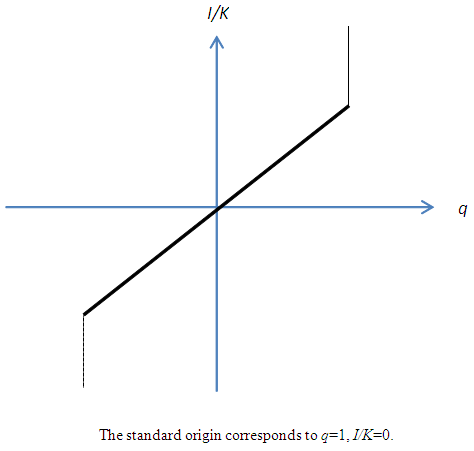
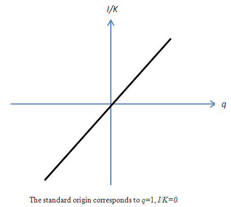 | Figure 1. Linear Investment Function Derived from the q Theory |
 | Figure 2. Non-linear Investment Function with an Insensitive Section to q (N-shaped) |
 | Figure 2'. Investment Function Degenerated from Figure 2: Complete Irreversibility |
 | Figure 3. Logistic-type Investment Function (S-shaped) |
4. Multiple q Theory and Its Augmentation to a Non-Linear Model
4.1. The Basic Framework of Multiple q
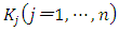
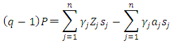
- Multiple q theory, which augments q theory to cases of multiple goods, provides the benchmark for an investment function that incorporates the heterogeneity of capital goods. Wildasin (1984) noted that in the multiple goods model, a monotonic one-versus-one relationship between simply totaled investment volume and average q did not hold any longer, but it was possible to uniquely determine average q as the function of the investment volume vector of each capital good. Asako, Kuninori, Inoue, and Murase (1989) named Wildasin's (1984) multiple goods model the “Multiple q theory,” and the conventional q theory that assumes single totaled capital goods the “Single q theory,” They used financial data from Japanese listed firms in the manufacturing industry and carried out an empirical analysis of the investment function based on Multiple q that consisted of two capital goods, land and depreciable fixed assets.29 In this analysis, as will be seen later, the average q of Wildasin (1984) was renamed “Total q” targeting all of the multiple capital goods by Asako et al. (1989). Asako et al. (1989) aimed to clarify the characteristics of land investment, which is the greatest feature of investment behavior in a bubble economy then going on in Japan. As the continuance of this, Asako, Kuninori, Inoue, Murase (1997), who analyzed data up to 1994, precisely constructed data on the market value of land owned nationwide by firms. In contrast to this, targeting data up to 2004, Tonogi, Nakamura, and Asako (2010) instead of simplifying the assessment of land, analyzed depreciable fixed assets in detail by subdividing them into four categories; buildings and structures; machinery and equipment; vessels and vehicles; and tools, furniture, and fixtures. In addition, through comparing the estimation results from the three kinds of methods for constructing capital investment and capital stock data (as will be described later, the proportional method, the book value method, and the zero method), they indirectly verified how behavior for the new acquisitions of capital goods and for sales and retirements of those differ. The main conclusions of Tonogi, Nakamura, and Asako (2010) were as follows. First, insofar as assuming a smooth convex adjustment cost function, the Multiple q investment function incorporating the heterogeneity of capital goods performed better than Single q.30 However, even the Multiple q framework had unsatisfactory explanatory power, particularly so in cases of net investment (the net of new acquisitions and sales and retirements). Second, even in the estimates targeting gross investment (new acquisitions only), for which the Multiple q framework’s explanatory power is relatively high, variables that should not have explanatory power in the q theory in which q is the sufficient statistic―namely, the cash flow ratio and interest bearing debt to asset ratio―were estimated as significant. This suggested that consideration of the heterogeneity of capital goods while maintaining the convex adjustment cost framework resulted in factors still remaining unexplained. Third, for differences in investment behavior according to capital goods, they found that behavior to new acquisitions of buildings and structures and of tools, furniture, and fixtures, takes place consistently with a smooth convex adjustment cost function, regardless of the time period. However, they obtained no significant result in a consistent form for behavior to new acquisitions of other capital goods, such as machinery and equipment, or for sales and retirement behavior as a whole. Based on this, Asako and Tonogi (2010) allowed the adjustment cost function to have the non-convex part that results in the lumpy and intermittent/infrequent investment, and estimated the augmented Multiple q type investment function. Specifically, they had in mind the combination of the fixed-costs part and convex adjustment costs, and considered two models; an “inner-fixed-outer-convex” type model that severs the correlation between the investment rate and q in the area where it is normally assumed that the absolute value of the investment rate is small and that becomes a N-shaped investment function with a jump (Figure 4)31; and as is shown in Figure 5, an “inner-convex-outer-fixed” type model that severs the correlation between investment rate and q in the area where the absolute value of the investment rate is large.32 For both models, the large and small threshold values of the investment rate that becomes non-continuous in the relation with q for each category of capital goods are to be estimated as the percentile values of the distribution of the investment rate. In practice, as these threshold values cannot be estimated directly, they exhaustively estimated the investment function for each candidate combination of percentile values for each category of capital goods in the manner like the grid search method, and then choose the case which records highest coefficient of determination as the estimates of threshold percentiles. However, Asako and Tonogi (2010) only provided an overview of this using a fairly rough grid as their main purpose centered on the hypothesis testing of the heterogeneity of capital goods. In this section, following the method of analysis of Asako and Tonogi (2010), a more detailed grid will be used and the non-continuity of the investment function of each capital goods will be clarified.
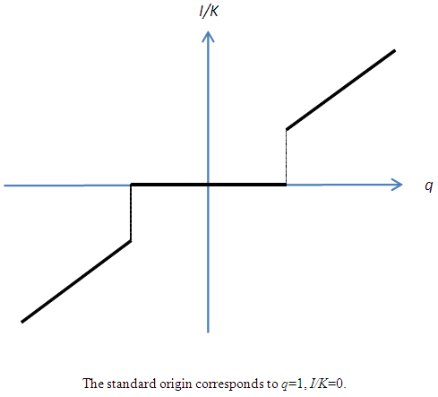 | Figure 4. Example of Inner-fixed-Outer-convex Investment Function (N-shaped with Jumps) |
 | Figure 5. Example of Inner-convex-Outer-fixed Investment Function |
4.2. From the Linear Model to the Non-linear Model
- The non-linear multiple q model used in this section was developed based on perfect competition and constant returns to scale that are assumed by standard q theory with an additional hypothesis regarding the non-convexity of the adjustment cost function that results in the non-continuity of the investment function. Below, an overview of the model is provided by extending the comprehensive adjustment cost framework discussed in Subsection 3.1 to the multiple capital goods model.33 However, unlike 3.1, here the “beginning-of-period model” is adopted regarding capital accumulation. Namely, it is assumed that investment during the period all becomes productive capacity at the beginning of the period and so contributes to production in the current period.There are n classifications of capital stock and the capital goods' number
 at the end of the previous period is written by
  , where
  as before denotes each capital good's physical depreciation rate. To be rigorous, capital stock after the investment at the beginning of the current period is
  , and capital stock at the end of the current period is
  . Then capital investment is expressed by
  . The differences between this “beginning-of-period model” and the “end-of-period model” in Subsection 3.1 are not intrinsic in theoretical terms. Tonogi, Nakamura, and Asako (2010) estimated both, with the performance of the former being the clear winner. Therefore, as part of this series of research, here, the “beginning-of-period model” is adopted. The Cobb-Douglas type functional form, i.e.,
  with non-negative parameters
  is assumed for the firms’ gross profit function. The convex adjustment cost function of investment can be separated for each capital goods, and first, as the base line model, it is assumed to be the multiplication of two parts. One is the quadratic function of the investment rate
 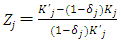 relative to the capital stock at the end of the period, and the other is the scale of capital stock at the end of the period
  . In sum, the expression becomes as follow:
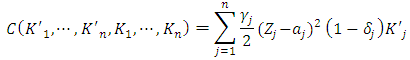 | (7) |
 is the parameter that controls the size of the adjustment costs of investment, and as is shown below, plays an important role in terms of characterizing the investment function based on Tobin’s q theory. The parameter
  represents the investment rate in which adjustment costs take the minimum value, and adjustment costs increase gradually the more the investment rate diverges from
  . Generally, for
  , which becomes the benchmark, it is natural for it to become 0, as in the single goods model developed in Subsection 3.1, or in the neighborhood of the capital depreciation rate
  . However, in this section, it is empirically estimated.34Under the assumptions made above, the Bellman equation for the maximization problem for firm value V, with β as the discount factor and E as the expected value operator, is expressed as follows.
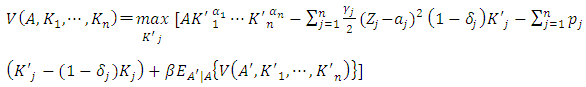 | (8) |
 denotes the price of capital good j relative to the product price as the numeraire. From the envelope theorem, when equation (8) is differentiated and arranged with regards to
  , we obtain the firm value maximization condition
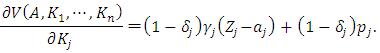 | (9) |
 , by Euler's theorem for the homogeneous function,
 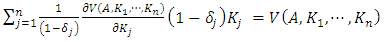 | (10) |
 where
where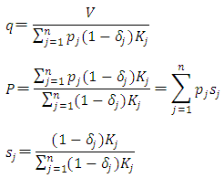 | (11) |
 is the share of each capital good as a percentage of totaled capital stock, and is also the weight when investment rate is totaled over heterogeneous capital stock. Generally, estimation of the investment function using the Multiple q framework uses the system of equations (11) that includes the definitions of the variables. First, with
  as the explained variable and
 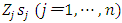 and
and  as the explanatory variables, linear regression is carried out and estimates obtained of
  and
and  , which are adjustment cost function’s coefficient parameters. Subsequently,
  and
and  are identified for respective capital goods.35Above, an overview of the Multiple q model based on the standard convex adjustment cost function was provided. Below, upon permitting the non-convexity of adjustment costs, equation (7) is revised as follows.
 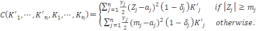 | (12) |
 reaches
  , it is assumed only the fixed amount applies to the investment adjustment costs, and when
  is exceeded, quadratic (convex) adjustment costs are additionally generated for the investment rate for this excess part. This is the “inner-fixed-outer-convex” model described by Asako and Tonogi (2010).36As the opposite of this, we can also consider another type of non-convexity, in which in the area where the absolute value of the investment rate is small, the usual quadratic (convex) adjustment costs apply, but even when it is exceeded, additional adjustment costs are not generated. The adjustment cost function in this instance can be expressed by replacing
  in equation (12) with
  . This is the “inner-convex-outer-fixed” model described in Asako and Tonogi (2010).37 If we were to intuitively express the differences between the “inner-fixed-outer-convex” and “inner-convex-outer- fixed” types, the unresponsive area of investment rate with regards to q (in other words, the area that cannot be explained by q) in the former is assumed to be small-scale investment, as is shown in Figure 4, while the latter is assumed to be large-scale investment, as is shown in Figure 5.
 4.3. Data Construction and Method of Empirical Analysis
- The data set used for the estimation was the same as used by Tonogi, Nakamura, and Asako (2010) and by Asako and Tonogi (2010). Based upon the data from the individual financial statements of firms listed on the first and second sections of the Tokyo Stock Exchange, Osaka Stock Exchange, and Nagoya Stock Exchange that has been collected in the DBJ Database of Listed Firms (DFDB) of the Development Bank of Japan38, a non-balanced panel data is constructed for all periods insofar as there is data on delisted firms and newly listed firms.39The investment amount is theoretically defined as “the amount of the new acquisitions of capital goods” minus “the residual market prices of sales and retirements of capital goods.” However, there does not exist any observable data on the residual market prices of sales and retirements of capital goods, and moreover, the data that can be used for estimations is limited. Therefore, in previous research, roughly speaking three kinds of facile methods have been used. The first is a method of obtaining a value in which the “current price-book value ratio” is multiplied by the book value of the amount of sales and retirements obtained from a reverse operation from the identity equation in accounting (subsequently called “the proportional method”). This method was adopted in research including Asako, Kuninori, Inoue, and Murase (1989, 1997) and Hayashi and Inoue (1991). Second is a method that uses unchanged book value of sales and retirements obtained from a reverse operation from the identity equation in accounting (subsequently called the “book value method”). This method was adopted in research including Suzuki (2001). In the third method, it is uniformly set as zero emphasizing the merit of avoiding the noise brought by measurement errors over the demerit of losing information of sales and retirements which is usually little compared to new acquisitions (subsequently called “the zero method”). In addition to Hori, Saito, and Ando (2004), this method has frequently been adopted in overseas research, including those introduced in an earlier section. As another interpretation of the zero method, the sales and retirement amount might be thought to be included in depreciation and amortization as a fixed ratio of existing capital stock. Of course, this interpretation can be criticized for ignoring non-periodical and large-scale sales and retirements. If we compare and contrast the above three methods, it should be noted that if we estimate the investment function using investment data from the zero method, the results of the estimates will only reflect behavior to new acquisitions of capital goods. In contrast, when using data from the other two methods, behavior to sales and retirement of capital goods is also incorporated into the analysis.40 From the classifications of depreciable fixed assets collected as the schedule of property, plant and equipment in the DFDB, when noncurrent fixed assets for rent and other depreciable assets that are outside the scope of the analysis are excluded, we are left with six classifications; buildings; structures; machinery and equipment; vessels (including aircraft); vehicles; and tools, furniture, and fixtures. Within these six, the correlation of the investment rates of buildings and structures is high, and also, with regards to vessels and vehicles, not many firms own vessels; therefore, they were respectively grouped and treated as single capital goods. Also, in the Multiple q empirical research of Asako, Kuninori, Inoue, and Murase (1989, 1997), Tonogi, Nakamura, and Asako (2010), and Asako and Tonogi (2010), land was also treated as a capital good with inherent adjustment costs for investment, and it is treated the same way in this paper. In the end, capital investment and capital stock data are classified into the five classifications of capital goods of “buildings and structures,” “machinery and equipment,” “vessels and vehicles,” “tools, furniture, and fixtures” and “land”, and the calculations are performed using each of the three methods mentioned above. With regards to average q (total q), in the case of actually existing firms, firm value includes market value of assets other than the capital stock in the five classifications described above. Therefore, by subtracting this part, conformity with the theoretical model is maintained. Assuming that the current prices of liabilities and assets other than the capital stock are equal to the book values, then q can be expressed as follows.
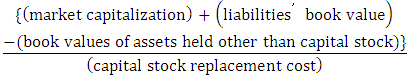 where market capitalization on the numerator equals the market value of stock price and assets held other than capital stock is evaluated by book value. Note that, as the beginning-of-period model is assumed, these values are all measured at the beginning of the period.There are four sample periods in estimating the investment function, which are shown below: (1) first period, fiscal 1982 to 1986 (pre-bubble economy period),(2) second period, fiscal 1987 to 1991 (the bubble economy period),(3) third period, fiscal 1992 to 1997 (the period after the collapse of the bubble economy),(4) fourth period, fiscal 1998 to 2004 (the financial crisis and recovery period). As these periods were divided based on the features of investment and capital stock by each category of capital good as well as the changes to Total q and the economic situation,41 it should be noted that the lengths of all of the sample periods are not uniform. We took the following steps to estimate the threshold forming the boundary between the fixed and convex portion: in the case of the inner-fixed-outer-convex type (inner-convex-outer-fixed type), we compared the best fit of the estimation equation (coefficient of determination) using the combination of the 5 capital goods, for any of the 10 symmetrical pairs of investment rate distribution, separated by percentiles, in 5% intervals where the interior (exterior) represents fixed cost, i.e. (0%, 100%) (5%, 95%)... (40%, 60%) (45%, 55%). This determined the optimal interval from among 105 combinations (See Figure 6).42 Using this as a base case, we tested other variations including cases where the inner-fixed-outer-convex and the inner-convex-outer-fixed types are mixed depending on goods. We used OLS for the estimation method. We have reported the results of the fixed effects model in all cases, taking into account the results of the Hausman test.43
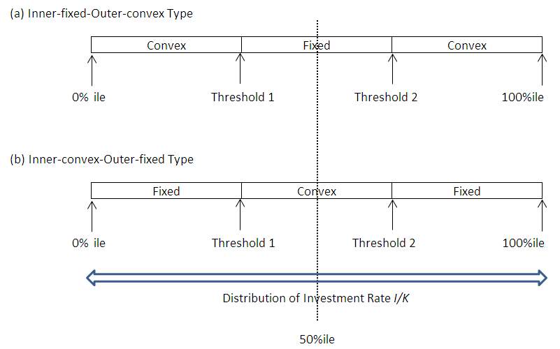 | Figure 6. Estimated Boundary Value (Percentile) of the Convex and Fixed Portions: Base Case |
5. The Main Estimation Results and Implications of the Non-linear Multiple q Model
5.1. Estimation Results of the Base Case
- Table 1 shows the inner-fixed-outer-convex type and inner-convex-outer-fixed type for each estimation result based on the basic form (combinations of the percentiles that maximize the coefficients of determination).44 Due to repeated references in the text, hereafter we will refer to the inner-fixed-outer-convex type as the "inner-fixed type," the inner-convex-outer-fixed type as the "inner-convex type."One item that can be generally pointed out is that the introduction of non-linearity improves fit. In other words, with the exception of the inner-fixed type, zero method, and the first estimation period, the coefficient of determination increases in comparison to the usual Multiple q model which assumes convex adjustment cost across the entire investment rate.45 In addition, when we view this increase by estimation period, overall there is a large improvement in fit in the second and third periods from the introduction of nonlinearity, and in particular there is noticeable improvement in the following: for the second period, the proportional and book value methods, which integrated the sale and retirement of equipment; and in the third period the zero method, which captured only the new acquisition behavior of equipment. As a whole, similar to estimations of all-convex type, the zero method is a better fit in comparison to the proportional and book value methods. However, when considering just the second period, the advantages of the zero method becomes quite small when considering nonlinearity. This may be related to the fact that the second period is centered around the bubble economy era, when there were relatively few sales and retirements.There is no absolute dominance by either the inner-fixed type or inner-convex type with regards to the goodness of fit, but since the coefficient of determination of the inner-fixed type only exceeds that of the inner-convex type 4 out of 12 cases, it can be said that relatively, the inner-convex type is dominant. Interestingly, in the first and the third periods, the inner-convex type is superior in all three methods, while, in the second period, the inner-fixed type is superior for all three methods. The difference caused by timing is prominently seen. The second period is considered to be the estimation period with many large-scale investments, but this can be explained by the usual convex adjustment cost, rather than the lumpy investment model. However, we must be wary of the possibility that stock prices at the time may have included elements of an economic bubble. Next, we take a look at the intervals corresponding to the fixed costs selected in each of the inner-fixed type, inner-convex type models. First, naturally the scope of the investment rate is completely different according to definition, but the selected percentiles for the proportional and book value methods, which integrated the sale and retirement of equipment, largely deviate from that of the zero method which captures only new acquisitions of equipment. This trend is particularly strong for the inner-fixed type, and inconsistent results can be spotted even between the proportional and book value methods.Within the inner-fixed type, the new acquisition behavior of machinery and equipment (zero method) had relatively stable results. Specifically, the optimal case in the first and second periods was fixed costs for the entire area, and even in the third and fourth periods, fixed costs were optimal for (5%, 95%) or almost the entire area. As long as we assume the inner-fixed type, this suggests a very sparse relationship between new acquisition of machinery and q. On the other hand, if we look at the new acquisition behavior of buildings and structures, although the first period showed (30%, 70%), the second period onwards all showed (45%, 55%), where the fixed costs portion was narrow, and the portion explained by convex adjustment cost was broader. For buildings and structures, the selection results were nearly the same for either proportional or book value method. Of the five types of capital goods, the estimation results are particularly stable, as evidenced by the increase in fixed cost portion following the integration of the sale and retirement behaviors.46Next, when we look at the inner-convex type, fairly consistent results are obtained between the proportional and book value methods in each category of goods excluding vessels and vehicles. We do not see as large a deviation between the zero method as in the inner-fixed type. First, in buildings and structures, a very narrow range of percentiles for fixed-cost parts or even all-convex were selected across the three methods and four periods. Tools, furniture, and fixtures shows a similar trend although with some exceptions. These results are consistent with Tonogi, Nakamura, and Asako (2010) which postulated all-convex adjustment cost, and which most significantly estimated the new acquisition behavior of these two categories of goods. On the other hand, with regards to machinery and equipment, there is large variation by period in the zero method, but the proportional and book value methods almost entirely select all-convex or (5%, 95%). In Tonogi, Nakamura, and Asako (2010), the performance of estimations in machinery and equipment have generally not been favorable, but there is a possibility that the goodness of fit improved through the consideration of the fixed portion. For land, the intervals of the fixed portions are slightly wider than for machinery and equipment, but nearly the same results are obtained in the proportional and book value methods.So far, we have viewed the characteristics of the estimation results in the base case. What should be noted is that a significant proportion of cases have selected (45%, 55%). In particular, the trend is represented strongly in the inner-fixed type. In all methods and estimation periods, with the exception of the first period in the proportional method and the second period of the book value method, have this percentile in some category of capital goods. In addition, in the inner-convex type, this percentile is selected in 5 out of 12 cases for some category of capital goods. The percentile (45%, 55%) is one step short of (50%, 50%), that is, on the verge of all areas to be convex in an inner- fixed-outer-convex type, and all areas to be fixed in an inner-convex-outer-fixed type.47 In the base case, in order to compare the merits and demerits of the inner-fixed and inner-convex types, we set the search range from (0%, 100%) - (45%, 55%) under the constraint that all category of capital goods belong to the same type. Thus (45%, 55%) has signified a type of boundary solution, and the fact that this has been selected many times suggests the possibility for the capital goods in the inner-fixed and inner-convex types to be intermingled. Therefore, we will next try an intermingled case.
5.2. Estimation Results of the Inner-fixed and Inner-convex, Hybrid Type
- The inner-fixed, inner-convex hybrid type requires immense amounts of computation, and so we set the increments of the grid to 10%. Table 2 shows the estimation results.Firstly, in exclusion of the first-period, proportional and zero methods, which selected the percentile of the inner-convex type in all categories of capital goods, the 10 out of 12 cases selected combinations where the capital goods of the inner-fixed and inner-convex types were intermingled. As a general direction, this backs the prediction in the preceding paragraph. However, the coefficient-of-determination levels show only a small amount of improvement, if any, when compared to the maximum estimation value of the base case (with no intermingling). Even if discounting the negative impact from increased grid increments, it is hard to judge this is a significant change. Additionally, of the 5 goods × 12 cases = 60 sets of percentiles, 39 of the sets selected the inner-convex type (except when equivalent listings selected different types). In the comparison between the inner-fixed and inner-convex types, similar to the base case, the inner-convex type is relatively superior.Next, when we view each category of capital goods, the percentiles of the inner-convex type is selected in the following cases: in machinery and equipment, 11 out of 12 cases excluding the fourth period of the zero method; in tools, furniture, and fixtures, 10 out of 12 cases excluding the second periods in each book value and zero methods. Basically the investment behavior of both capital goods may be explained consistently by the inner-convex type. In other words, in absolute values, q theory fits in an investment rate of a set range, while there are also large new acquisitions, sales, and retirements which cannot be explained by q. In contrast, the inner-fixed type is dominant for the proportional and book value methods of vessels and vehicles. In absolute values, the investment rate of a set range is carried out independent of q, but for large new acquisitions, sales, and retirements, q theory fits. With respect to buildings and structures and land, it is difficult to point out distinct characteristics such as those described above.Moreover, if we view the characteristics by estimation period, the inner-convex type is particularly dominant in the first period, and the majority of selected percentiles are those with narrow external fixed portions. In addition, the dominance of inner-convex type is also significant in the third period except for vessels and vehicles. The majority of selected percentiles, when excluding land, are those with narrow external fixed portions. In contrast, in the second and fourth periods, the inner-fixed types have also been selected correspondingly. The second and fourth periods represent times when stock prices reached extreme pessimism and optimism (the fourth period includes a period of optimism during the IT bubble), and it may also be interpreted that the investment rate of a set range was carried out calmly and independently of these moves.
5.3. Estimation Results of other Derivative Cases
- The estimation thus far has assumed that, either in the base case or in the hybrid type, the 3 intervals bounded by the 2 thresholds would appear in symmetrical form at the center of the investment rate distribution. On the other hand, a model is also conceivable whereby the assumption is removed requiring symmetry on both sides, and the width of the middle interval of the 3 is set to 50% and the thresholds are shifted by 5 percentile to the left and right (width 50 percentile fixed model).Estimating this model on each the inner-fixed type and inner-convex type, we obtain the results in Table 3. Here, we eliminate the case to degenerate into the two intervals with one of the threshold values becomes 0 or 100 percentile. First, we compare the coefficients of determination in the inner-fixed and inner-convex types. Similar to the base case, the inner-convex type is relatively dominant in the proportional method. On the other hand, in the book value and zero methods, the inner-fixed type is superior. However, in comparison to the coefficients of determination of the basic model, of the total 24 cases of inner-fixed and inner-convex types, the only case where a fixed-width model became relatively superior was the inner-fixed type, book value method, and second period. Therefore we can see that the reason the inner-fixed type became superior in the fixed-width model, was only that its coefficient of determination declined less than that of the inner-convex type. This suggests that the previous assumption is correct in setting a bilateral symmetry centered on the 50 percentile to find the "position" of the middle interval of the 3 intervals, and suggests that the selection of "width" is more important.However, looking at the percentiles selected in Table 3, we can see that (5%, 55%) and (45%, 95%) account for a large proportion of both the inner-fixed and inner-convex types. Since we eliminate cases where one threshold is 0 or 100 percentile, these are regarded as the "boundary solution." This suggests the importance of considering that one of the thresholds may be absorbed by the edge of the distribution.Lastly, we removed the assumption of fixed width and estimated 2 cases, a degeneration into binary patterns (upper & lower) by a single threshold, that is, the "lower-fixed type" where the lower portion of the distribution is fixed and the upper portion is convex, and the "upper-fixed type" where the lower portion of the distribution is convex and the upper portion is fixed (Table 4). Taking the higher of the upper-fixed and lower-fixed types, the model's coefficients of determination exceed the inner-fixed, inner-convex hybrid type model with bilateral symmetry, which previously had the highest coefficients of determination, in 11 out of 12 cases excluding the third period of the zero method. In the proportional and book value methods, the assumption of bilateral symmetry means that the same model will be applied for both large-scale new acquisitions and sales/retirements. But the fact that there is a higher coefficient of determination for the upper-fixed and lower-fixed types, suggests that rather, it is better to fit different models for large-scale new acquisitions and sales/retirements.If comparing the coefficients of determination between the upper-fixed and lower-fixed types, the latter has a higher figure, with 9 of the 12 cases. However with regards to this model, the following points are more important than a comparison of the two types. The intervals of the fixed portion suggested by the upper-fixed and the lower-fixed types include cases where completely consistent results are obtained, like in periods 1 and 3 of buildings and structures in the zero method, or periods 1, 3, and 4 of tools, furniture, and fixtures in the zero method, while some cases have completely inconsistent results. “Completely inconsistent” refers to the situation where the threshold values are the same but the convex and fixed portions are completely interchanged, such as in periods 1 and 2 of land in the proportional method, where the upper-fixed type model obtains the results, 0-90% in the convex portion and 90-100% in the fixed portion, while the lower-fixed type model obtains 0-90% in the fixed portion and 90-100% in the convex portion.48 In addition, there are even more cases where the threshold values have a slight deviation but where these types of interchanges occur. Overall, there is a tendency for broad estimation in the convex portion of the upper-fixed type and broad estimation in the fixed portion of the lower-fixed type.At first glance this situation seems difficult to interpret. However, even in completely inconsistent cases, if we focus on the fact that the estimated threshold itself is consistent, then the results are by no means inexplicable. In other words, we obtain consistent estimation results with respect to the boundary for changes in investment behavior, but the selection of which side to apply the convex differs per model. Considered this way, we can see that the threshold of changes in investment behavior for "inconsistent" cases is roughly 70%ile to 100%ile, namely the upper portion of distribution of investment rate or the range of large-scale investments. In a world of binary patterns, consider the case that convex adjustment costs fit either portion but parameters differ between two portions. Then apparently it is difficult to explain everything using one convex adjustment cost function. Thus it is conceivable that consequently, either was estimated as the fixed portion.As described above, what was revealed from the estimation results of the Multiple q model investment function which allowed for the non-convexity of adjustment costs, was that there is a clear difference in the appropriate functional type, dependent on whether capital goods, estimation periods, and whether new acquisition and sale/retirement are regarded as integral actions. This fully supports the process in which Cooper and Haltiwanger (2006), who had used undifferentiated capital investment data (in terms of capital goods) to carry out the estimation of comprehensive investment functions encompassing as special cases the main models of capital investment research subsequent to the q-theory had arrived at their conclusion, that "the differing types of capital have differing and corresponding processes of adjustment."
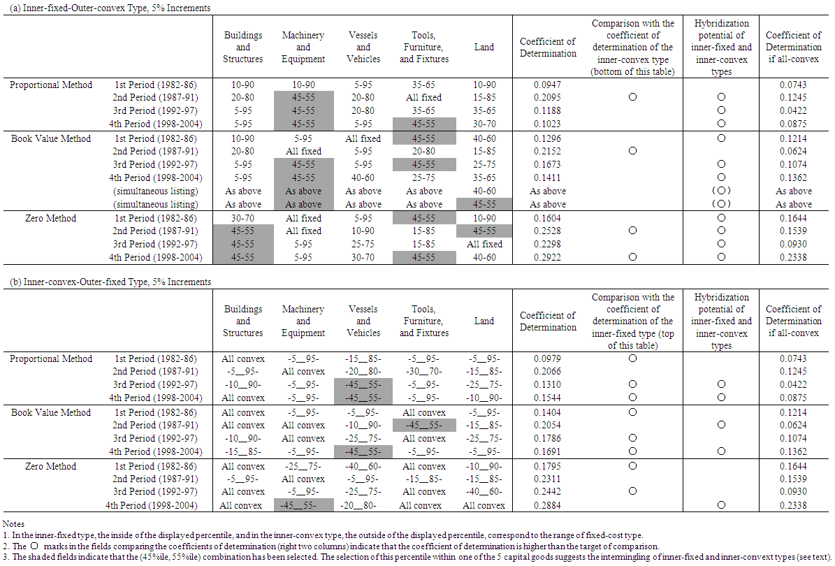 | Table 1. Estimation Results of the Base Case: the Percentiles that Maximize Coefficients of Determination |
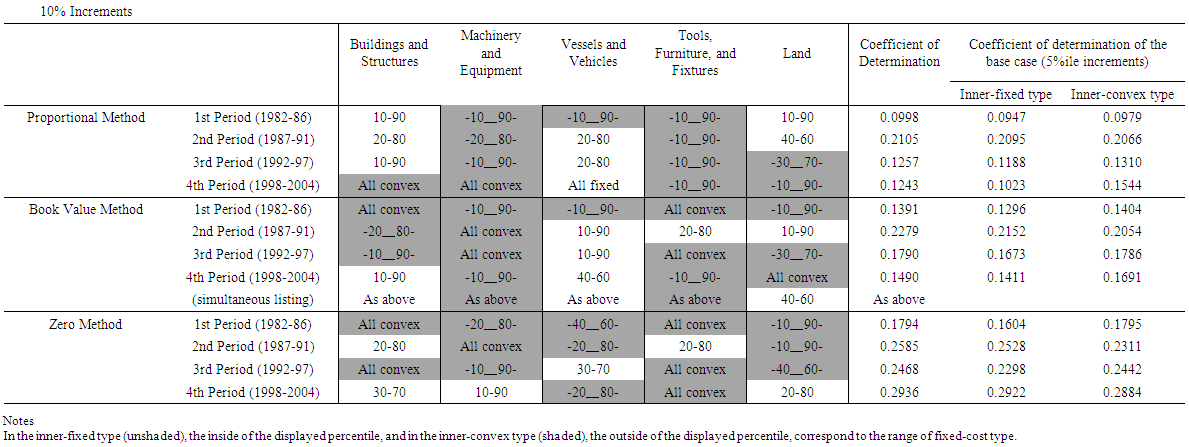 | Table 2. Estimation Results of the Inner-fixed / Inner-convex Hybrid Type: the Percentiles That Maximize Coefficients of Determination |
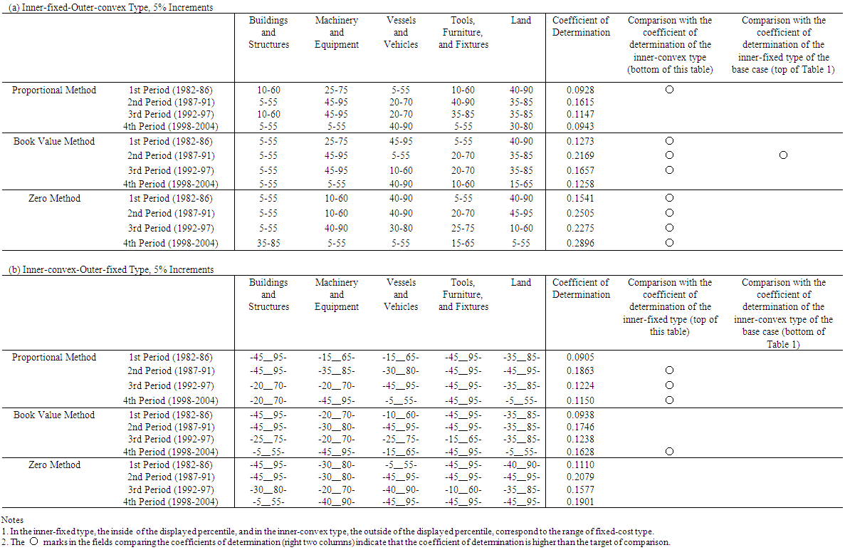 | Table 3. Estimation Results of the Fixed Model with 50%ile width: the Percentiles That Maximize Coefficients of Determination |
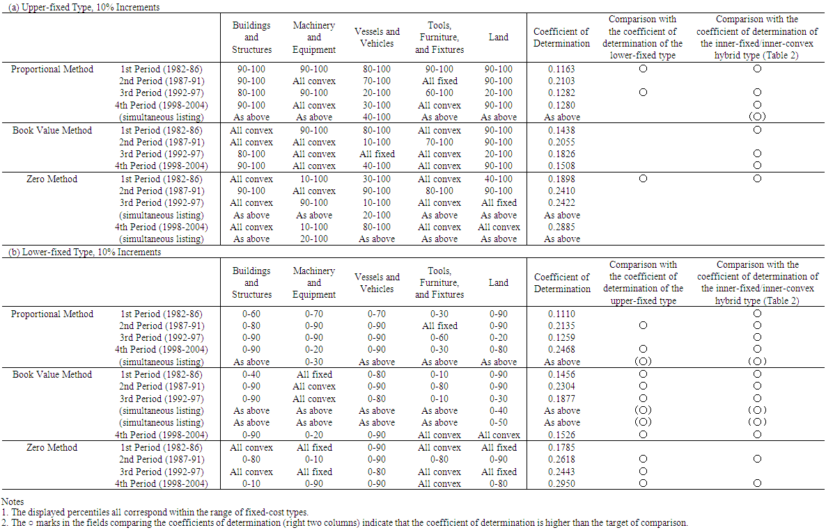 | Table 4. Estimation Results of the 1 Threshold Model: Percentiles that Maximize Coefficients of Determination |
6. Conclusions
- In the first half of this paper, we looked back at a gallop the development of capital investment research in the 25 years since Asako and Kuninori (1989). Its starting point was that the empirical performance of q-theory, a theory rooted in neoclassical microeconomic foundations and which had been looked to as the culmination of investment theory to unify traditional investment functions, had been unable to live up to expectations. To overcome this, the investment model has made a variety of developments accompanied by new empirical findings obtained from micro data on an establishment level, and research has accumulated in a remarkable speed.However, these developments have not overwritten all former discussions. The convex adjustment cost function assumed by q theory still coexists as an essential element in describing investment behavior along with new theories such as lumpy, intermittent investment. We had not emphasized this so far, but one of the reasons includes the difference in the level of aggregation with respect to the investment entity. For example, a recent, dynamic general equilibrium macroeconomic model incorporates the investment function (so-called CEE model) proposed by Cristiano, Eichenbaum, and Evans (2005) that is considered to have high consistency with real data and employed as a standard. It is a function type that imposes a penalty to changes in investment level consistently with the convex adjustment cost, and because it can explain the influences of past investment levels (one of the anomalies regarding q-theory), it implies an investment behavior that is more sticky than q-theory, in contrast to the theory of lumpy, intermittent investment. According to Eberly, Rebelo, and Vincent (2011), the CEE model possesses a relatively high explanatory power with regards to the investment behavior of large companies, and as Doms and Duune (1998) suggested, there is a possibility that aggregation has leveled the lumpy, intermittent investment behavior on an establishment level.49In the second half of this paper, we conducted empirical analysis within the framework of Multiple q (an extension of q theory to the case of multiple capital goods), for important background themes with regards to the "coexistence" of new and old theories, such as the heterogeneity of capital goods, and the heterogeneity between new acquisition and sale/retirement in investment behaviors. The estimation results of the Multiple q model, which had been extended to include the possibility of the adjustment cost function containing a non-convex portion, have highlighted even more the variety of forms in investment functions, dependent on the types of capital goods, estimation period, and whether new acquisition behavior is solo or integrated with sale/retirement behavior. That is, while we observed a proportion of cases that fit purely-convex adjustment cost functions, we confirmed that on the whole the cases that included non-convex portions formed a majority, and even in this case, in the non-convex areas of the investment rate distribution, there was a large variation depending on the types of capital goods and estimation period. However, we have as yet tested only a small portion of possible processes of adjustment created by various forms of heterogeneity. So in closing, we present an overview of future research agenda for the empirical analysis of capital investment, using the Multiple q framework.Firstly, according to the implications from the estimations of the best-fitting models in the analysis thus far – the upper-fixed and lower-fixed types – the next step deserving of an attempt would be the estimation of models that apply 2 convex adjustment costs with differing parameters to each of the 2 intervals. Its performance will test the necessity of applying fixed-cost types. For example, if a case consisting of 2 types of convex adjustment costs are more desirable than a combination of convex and fixed types, then we may need to apply differing convex adjustment costs to the outer 2 of the 3-intervals based on inner-fixed-outer-convex type model. By continuing these sorts of searches, we believe we can identify models with higher explanatory powers with regards to the characteristics of adjustment processes of different capital goods.The second agenda is to perform an estimation that more explicitly incorporates nonlinearity, through the ease of the so-called "curse of dimension" problem. As seen so far, the financial data of Japan's listed firms disclose detailed information pertaining to capital stock, broken down by goods. This presents an ideal platform to analyze the heterogeneity of capital goods, however, this also poses a serious challenge in the limitations of computational resources when trying to analyze goods-based information while preserving its integrity as much as possible. For this reason, the nonlinearity of investment functions referenced in this paper is simply incorporated as forms that "do not fit a linear relationship with q." As in Cooper and Haltiwanger (2006)'s comprehensive adjustment cost function introduced in Section 3, in order to estimate a multiple-capital goods model that includes several types of nonlinearity more explicitly, one direction might be to conduct a factor analysis in advance to consolidate the dimensions of the capital goods without losing essential information.50The third agenda is the analysis of the adjustment process of the sale and retirement behavior by itself. In the past, we have analyzed the heterogeneity of new acquisition behavior and sales/retirement behavior through the data comparison between that of only new acquisitions, and the integrated data of new acquisitions and sales/retirements. This is an unavoidable method to obtain stable estimation results in the current situation, where sale/retirement samples are small and the possibility of a measurement error is considerably larger than new acquisitions. However, this method is an expediency and creates frustration in that it only indirectly analyzes sales/retirements behavior. By using the micro data in official statistics, as well as financial data accumulated since 2005 which had been previously excluded from analysis in the data sets used since Tonogi, Nakamura, Asako (2010), we should look for possibilities in constructing data that can withstand the analysis of sale/retirement behavior by itself.Finally, an important research agenda is to explore the possibility of extending the scope of capital stock as a semi-fixed factor of production. Conventionally, for example, it was not uncommon to conduct an estimation of the investment function in considering inventory as part of the capital stock.51 In the future, given the growing importance of intangible assets amid economic growth and corporate management, or the spread of leases for tangible fixed assets, perhaps these should also be considered part of the capital stock. This point is not limited to Multiple q but is a fundamental question posed for all of capital investment research, and where broad consideration from the field is anticipated.
Notes
- * This paper was first prepared for the 50th Anniversary conference, held in March 2013, of the Research Institute of Capital Formation (RICF), Development Bank of Japan. We would like to express our gratitude to various useful comments from a number of participants. However, any mistakes are solely the responsibility of the authors. Also, the opinions expressed in this paper are the individual opinions of the authors and do not represent the opinions of the organizations that they belong to. We thank JSPS for Grants-in-Aid for scientific Research B (24285062) with which we could promote our research plans smoothly. The Japanese original was published as Chapter 4 of the book; Horiuchi, A., M. Hanazaki, and J. Nakamura eds., “The Japanese Economy: Financial Development and Corporate Behavior in a Changing Environment,” University of Tokyo Press, 2014. Quite a few revisions have been made for the English version. Incidentally, Asako and Kuninori (1989) was written for the 25th Anniversary conference of the RICF.1. Also for countries other than Japan, in research that has focused on the heterogeneity of capital goods, data on the level of the firm or the industry is basically used.2. As was pointed out by Suzuki and Honda (2014), when considering capital investment and employment, there are probably only a few cases where the plant or establishment is the actual decision maker. Therefore, if focusing on the decision making of firms, it is considered appropriate that data on firms is used.3. The conditions are as follows; the production function and adjustment cost function are linear homogeneous, the product market is perfectly competitive, and factor prices and the discount rate are exogenous for firms.4. In the research that competitively compared empirical performance for competing investment models, the results have generally shown that the q type cannot win against the acceleration type and the Jorgensen type, though the latter two are merely special cases of the q type in theory.5. In the linear investment function, the q coefficient is equal to the reciprocal of the slope (or the tangent) for the quadratic adjustment cost function. In other words, the extremely small size of the q coefficient signifies that the adjustment cost is extremely large (that the adjustment speed is very slow). Shaller (1990) surveyed the empirical research that used data on the United States and pointed out that the estimated q coefficients were roughly in a range of 0.003 to 0.01.6. In addition, as a phenomenon peculiar to Japanese firms in the period up to the collapse of the bubble economy against the backdrop of banks’ financing with land as collateral, it has been pointed out that the amount of land assets held and land prices had a significantly positive effect on investment. See, for example, Ogawa and Kitasaka (1998).7. In the q theory framework, a major assumption is that stock prices correctly reflect the market value of capital stock as so-called fundamentals (the present discounted value of future cash flow). However, in reality, stock prices, even if on average they regress to the fundamentals, in the short run can be extremely volatile and contain a lot of noise. Further, it is not unusual for there to be a divergence from the fundamentals over the long run, such as in a bubble economy. In recent years, research has been persistently carried out toward proposing an method of improving average q that focuses on removing the distortions produced by stock prices. For example, Cummins, Hassett, and Oliner (2006) estimated firm value from present discounted value from analysts’ predictions of firms’ future earnings, and the significance of average q in linear investment function improved. Also, even among firms thought to be facing liquidity constraints, their results showed that the cash flow variable ceased to be significant. In addition, Philippon (2009) used arbitrage condition between stock prices and debt prices using the Black-Scholes-Merton model and proposed estimating firm value and also the average q from bond market information, and similarly was able to show improvements to empirical performance.Tobin (1969) attempted to formulate the argument in Chapter 12 of Keynes’ General Theory and considered that he tacitly assumed that the numerator of q is not a fundamental, but rather reflects “a state of long-term expectation” that moves easily. Consequently, Tobin himself, while quickly realizing that his own theory could be interpreted within a neo-classical framework, was negative toward this interpretation.8. Estimates of marginal q constructed using this method are frequently called “fundamental q,” following Gilchrist and Himmelberg (1995).9. Moreover, Ogawa and Kitasaka (1998) added a non-fundamental variable calculated from the difference between average q and marginal q to the list of explanatory variables for their investment function, and analyzed the possible effect that the bubble economy had on investment levels. In their estimates, after controlling for various effects on investment―for example, the effects of land assets being used as collateral―they found that the effect of non-fundamental variable was negatively significant. On the other hand, Chirinko and Schaller (2001) used aggregate data on the major firms in Japan between 1966 and 1991 and, as part of their various analyses on the existence of the bubble economy, conducted a test similar to Ogawa and Kitasaka (however, they did not consider land assets), and concluded the opposite, that the bubble economy pushed-up investment.10. Hubbard (1998) surveyed and summarized the typical results and criticisms of it. Also, Erickson and Whited (2000) applied corrections of measurement errors and robust estimators with regards to measurement errors and showed that even among firms experiencing financial constraints, the explanatory power of cash flow practically disappears.11. On the other hand, as it focused only on the first-order condition and did not use any information on the transversality condition, which is the sufficient condition in order for there to exist an optimal solution, theoretically, the efficiency of the estimator is considered to be inferior (Hayashi (2000)). It has also been noted that a disadvantage is that a situation is not established that results in a boundary solution, such as “zero investment” described later.12. As theoretical research on the effects of uncertainty on capital investment, Hartman (1972) and Abel (1983) first concluded that uncertainty promotes investment assuming firms in perfect competition with linear homogeneous neoclassical production functions. However, the notion that the suppressing aspect of uncertainty might be stronger has been dominant among practitioners. This became the starting point for a series of research arguments that incorporated investment irreversibility. Their main findings were summarized by Dixit and Pindyck (1994). Ultimately, theoretically speaking, depending on the prior assumptions both “promotion” and “suppression” are possible, but empirically it can be said as the rough consensus is that uncertainty’s suppressing effect on investment is stronger. Surveys of the research in this field have been provided in Suzuki (2001) and Nakamura (2003). Also, see Tanaka (2016) in this special issue.13.
 signifies that firm value takes a negative value, or in other words, excessive debt (not an excess of debt in the accounting sense, but economically). At the very least in the non-stochastic model, such firms should not be able to survive.14. The argument on lumpiness of capital stock adjustment on the macro level that aggregates the adjustment behavior on the level of individual firms is a completely different argument to that in this section. For example, if all firms adopt a wait-and-see approach with capital stock lower than the optimal level due to serious uncertainty that extends to the entire economy, when this uncertainty is eliminated, their adjustments will start all at once, and even if the adjustment behavior of each individual firm is in accordance with convex-type adjustment costs, lumpiness will be observed at the macro-level. In addition, a model that assumes a sort of externalities or strategic complementarities in the sense that an individual firm’s investment will improve the earnings environment of other firms through a demand effect and promote their investments, as well as a model that assumes the imperfect information or the inefficiency in corporate governance which induces “herd behavior” that is not necessarily optimal, can generate lumpiness on the macro-level investment.15. Ikeda and Nishioka (2006) carried out the similar verification using data according to industry in Japan.16. Research that carried out the similar verification using data according to listed firms in Japan is Shima (2005) and Miyagawa and Tanaka (2009). In the initial research into lumpy and intermittent/infrequent investment behavior, as represented by Doms and Dunne (1998) and Caballero, Engel, and Haltiwanger (1995), there were many researchers who stressed that inaction and lumpy adjustment are two aspects of the same series of phenomena. However, as was noted in the previous section, there exist counter arguments that insist both can theoretically be discussed as independent phenomenon, and in addition, that inaction and lumpy investment does not occur simultaneously in an empirical sense. For example, in the comments of Michael Woodford to Caballero, Engel, and Haltiwanger (1995), he points out that the data presented by Caballero et al. cannot be said to be evidence of lumpiness, but rather is consistent with an “intermittently continuousness adjustment model” through a combination of convex type adjustment costs and irreversibility. 17. This sort of assumption, that investment during the period becomes productive capacity at the end of the period, is called the “end-of-period model” following Tonogi, Nakamura, and Asako (2010). On the other hand, the assumption that all investment during the period becomes productive capacity at the beginning of period and contributes to production in the current period is called the “beginning-of-period model”. Of course, the process by which firms actually accumulate capital is not as simple as presented in these models, but the models that can be adopted for empirical analysis are normally limited to these two. The differences in the assumptions of the two models do not result in any essential differences in theoretical terms though, in terms of an empirical analysis, it is necessary to select the most appropriate one according to the characteristics of the data and the objectives of the analysis. For further details, refer to Tonogi, Nakamura, and Asako (2010). 18. Here, q is “expected q” at the beginning of the next period, as “the end-of-period model” is assumed for the accumulation of capital.19. In actuality, with regards to non-convex type adjustment costs, the opportunity cost type and the capital proportional fixed cost type are estimated separately. Namely, when estimating
  ,
,  is assumed and when estimating F,
  is assumed.20. Research that applied the same method to data on Japan’s automotive-parts industry is Uchida, Takeda, and Shirai (2012). In the results of their provisional estimates, none of the parameters of any of the types of adjustment cost were significant, which passively supports the model without adjustment costs.21. As is argued in the previous section, for the combination of investment irreversibility and convex type adjustment cost, while being kinked, the continuity of the function is maintained for the shape of the investment function, as shown in Figure 2. In contrast to this, for the combination of the fixed adjustment costs and convex type adjustment costs that is discussed in the Multiple q model, in the instant that q exceeds the zero investment area, the investment rate jumps from zero and becomes a discontinuous function of q, as is seen in Figure 4.22. The S-shape is made up of the part in which the investment rate becomes convex for q, such as (A) to (B) in Figure 3, and the part that is concave, like (B) to (C). However, in Barnett and Sakellaris (1998) the convex part is not clearly observed from the data. 23. Theoretically, capital investment is the amount for new acquisitions of capital goods minus the amount for sales and retirements, but because data on the amount of sales and retirements is both difficult to obtain and unreliable, frequently in empirical research the amount of new acquisitions is used as a proxy variable. Also, negative investment at the level of the firm is considered to frequently occur in the form of an abolition of a plant or establishment. But in individual data on the level of the plants and establishments, such cases are omitted from the sample and so are not recognized as negative investment.24. In the data used for the analysis, because only data on positive investment was collected, it becomes a shape similar to Figure 2´.25. Here, rather than a continuous N-shape such as in Figure 2, it is assumed to be a N-shape with a jump, such as in Figure 4.26. If the distribution of the threshold values is uniform, the aggregated investment function will be linear. 27. The same as with Caballero, Engel, and Haltiwanger (1995), instead of q, the gap between the optimal level of capital stock and the actual level (namely the divergence from the optimal level) was used. 28. However, taking into account that aircraft is one of the capital goods that have a well developed used market, it is considered to be possible for normal capital goods to produce a different result. 29. Here, as is indeed the case with an individual firm, land is also considered to be a capital good with fixed adjustment costs (a quasi fixed factor) when an investment in land is made.30. Regarding a statistical test of the heterogeneity of capital goods within the five classifications of capital goods, Tonogi, Nakamura, and Asako (2010) only tested whether there were any capital goods different than the others. But in addition, Asako and Tonogi (2010) conducted a more rigorous hypothesis testing from two perspectives; (i) whether each capital goods were homogeneous with capital goods totaled from the remainder, and (ii) whether each pair of two capital goods were homogeneous. Whichever the method, the null hypothesis, of the homogeneity of the five classifications of capital goods, was rejected.31. In Figure 4, the area of small absolute values of the investment rate is drawn as a flat line, representing inaction or zero investment. However, in the inner-fixed-outer-convex type formulation itself, the only condition that is imposed is that there is no correlation between the investment rate and q within the two threshold values of the investment rate. Therefore the possibility of it taking another shape is not excluded.32. In Figure 5, the area of large absolute values of the investment rate is drawn as a line that jumps in both an upward and downward direction, representing the lumpy investment. However, in the inner-convex-outer-fixed type formulation, the only condition imposed is that there is no correlation between the investment rate and q outside of the two threshold values of the investment rate. Therefore the possibility of it taking another shape is not excluded and it also does not contradict an S-shaped investment function, such as in Figure 2.33. Refer to Asako and Tonogi (2010) for details.34. Theoretically, the same as with the investment rate, any value can be taken within the range of
  , including a negative value. 35. In Tonogi, Nakamura, and Asako (2010), when looking at cases where
  is estimated to be positive and significant (convex type adjustment costs are supported), they reported that in many cases,
  took a positive value. 36. As the fixed costs part in equation (12) is also proportional to capital stock
  , the linear homogeneity with regards to
  of adjustment costs provided by the whole of expression (12) is maintained, and it does not go beyond the framework of q theory.37. Unlike the inner-fixed-outer-convex type, the formulation of the inner-convex-outer-fixed type does not satisfy overall convexity, and therefore the formulation itself departs from the q theory framework. However, if it corresponds to the appropriate condition of investment’s marginal revenue, the possibility remains that it will not contradict to maximize firm value. 38. Detailed data on tangible fixed assets according to capital goods and according to increases and decreases, which is indispensable for estimates in the Multiple q model, is all collected in the DFDB if said data has been disclosed in a securities report.39. Tonogi, Nakamura, Asako (2010) and Asako and Tonogi (2010) are to be referred for the details on each of the following that are not mentioned in this paper: treatment of fiscal periods; deflators according to capital goods, including land; the rate of physical depletion of capital stock; the source of each data set; and the processing of outliers.40. As three series of capital investment data are used for the calculation of capital stock by the perpetual inventory method, there concurrently exists three series of capital stock data.41. They are described in detail in Tonogi, Nakamura, and Asako (2010) and Asako and Tonogi (2010), so we will not repeat them here.42. Asako and Tonogi (2010) only conducted estimations in the 3 symmetrical intervals separated by percentiles in 10% increments (0%, 100%), (10%, 90%), (20%, 80%). Additionally, from the percentiles, it is possible to specifically calculate
  the threshold of the investment ratio in equation (12), but we leave this for future discussion since this would require the verification and specification of the probability distribution function conformed by the investment rate.43. Among others, the basic settings are the same as Tonogi, Nakamura, and Asako (2010), and Asako and Tonogi (2010), for example the inclusion of the cash flow ratio and the interest-bearing debt ratio as additional explanatory variables. We included the cash flow ratio and interest-bearing debt ratio, not for verification of the financial constraints hypothesis, but to control unresolved problems in estimation as outlined in Section 2, such as measurement error.44. The coefficient of determination was calculated to the 11th decimal place, and allowed for a simultaneous listing if this still caused multiple percentile combinations to line up.45. However, for the inner-convex type, it is self-evident that the coefficient of determination will rise since, in including the all-convex type as a special case, it selects the optimal item.46. A larger portion of buildings and structures are explained by the convex adjustment cost than machinery and equipment and has higher robustness of estimation results. This is not consistent with the empirical studies using data from the United States and Italy, as shown in Section 3.3. However, we cannot make a simple comparison as, in our data set, “machinery and equipment” and “tools, furniture, and fixtures” are treated as different capital goods.47. In actuality, many of the inner-fixed type cases where (45%, 55%) was selected as the fixed portion, selected all-convex or a similar percentile in the inner-convex types. 48. In cases where such phenomenon occurs, there is a tendency for the fixed portion indicated by the inner-fixed type to be inconsistent with the fixed portion indicated by the inner-convex type for estimation results of the base case (Table 1). For example, in the first period for land in the proportional method as shown in Table 1, the fixed portion indicated by the inner-fixed type is a 10-90 percentile interval, whereas the fixed portion indicated by the inner-convex type is an interval of 0-5 percentile and 95-100 percentile.49. Interestingly, they have proposed another possibility with very practical factors, described as follows: when a senior manager (with authority to make a final decision on an investment project) assesses the investment budget of each establishment, they set the previous year's budget as the starting line, and the larger the divergence from the previous year, the lower the probability of budget approval.50. For example, Tonogi, Nakamura, and Asako (2014).51. For example, Hayashi and Inoue (1991).