Petros Katsis1, Thomas Papageorgiou1, Leonidas Ntziachristos2
1Emisia S.A, Antoni Tritsi 21, Service Post 2, Thessaloniki, GR-57001, Greece
2Laboratory of Applied Thermodynamics, Aristotle University of Thessaloniki, P.O. Box 458, GR 54124, Thessaloniki, Greece
Correspondence to: Leonidas Ntziachristos, Laboratory of Applied Thermodynamics, Aristotle University of Thessaloniki, P.O. Box 458, GR 54124, Thessaloniki, Greece.
| Email: |  |
Copyright © 2012 Scientific & Academic Publishing. All Rights Reserved.
Abstract
This paper presents a detailed methodology for the calculation of CO2 tailpipe emissions of advanced vehicle technologies such as hybrid, plug-in hybrid vehicles and similar range-dependent powertrains with respect to trip and mileage distribution. The concept is based on the realisation that advanced vehicle technologies require a more thorough knowledge of trip distribution characteristics based available statistical data rather than average trip length which is already used for cold and evaporative emissions calculation. The proposed discrete trip distribution modelling takes into consideration the unique characteristics of different technologies without adding too much complexity. Results show that this approach can provide a representative projection of the impact on energy consumption and CO2 estimation depending on the assumed trip distribution especially if crucial characteristics such as the average speed and state of charge are also considered in parallel. Closed form solutions for the simplified representation of indicative statistical trip distributions are extracted.
Keywords:
Mileage, Trip Length Modelling, Energy Consumption, Emission Factors
Cite this paper: Petros Katsis, Thomas Papageorgiou, Leonidas Ntziachristos, Modelling the Trip Length Distribution Impact on the CO2 Emissions of Electrified Vehicles, Energy and Power, Vol. 4 No. 1A, 2014, pp. 57-64. doi: 10.5923/s.ep.201401.05.
1. Introduction
The European Commission has presented the White Paper on Transport[1] which is a roadmap document setting the targets for the evolution of transport in the European Community until 2050. Key policies in the area are addressing CO2 emissions and energy efficiency in order to provide the fundamental mechanisms to decouple transport growth from fossil fuel consumption. For instance, the 20-20-20 is a collection of robust policies[2] aiming to achieve 20% lower CO2 emissions in 2020 compared to 1990.Within this framework, electricity stands out as an appealing candidate when it comes to decarbonisation strategies. The term electromobility (or e-mobility) often refers to the concept of using electric powertrain technologies and infrastructures to enable the electric propulsion of vehicles and fleets. E-mobility is mainly intended for passenger cars and light commercial vehicles as efficiency drops with mass increase. Hybrid electric vehicles (HEVs), plug-in hybrid electric vehicles (PHEVs), battery electric vehicles (BEVs), EVs with range extender (EREVs) and Fuel-Cell EVs (FCEVs) are some representative electromobility technologies which can, up to a different extent, minimise or even eliminate oil dependency and tailpipe CO2 emissions, provided that the production supply chain does not emit too much CO2. On the other hand, HEVs, PHEVs and EREVs can maintain current conventional vehicle ranges, but do not allow full oil independency unless renewable fuels are used; while modern battery EVs have low electric ranges due to limitations of the battery storage capacity. It is quite apparent that there several similarities and several differences among these technologies.Furthermore, it is possible that other advanced technologies, either in the form of targeted eco-innovations or as new vehicle types will enter the market in an attempt to achieve the agreed targets. Therefore, it should be investigated whether these different technologies can be modelled with the currently available tools and methodologies used for conventional vehicle technologies.One parameter which is important for the modelling of such vehicles is the trip length distribution. For conventional vehicles, average trip length is an important parameter for the estimation of emissions in vehicles due to the influence on the cold start excess. It also plays an important role in the estimation of evaporative emissions.However, with the introduction of advanced technologies in transportation, the trip length distribution received additional importance. In such cases it plays a decisive role as it may indicate the ranges in which the new technology cars will operate in a special mode (e.g. all-electric mode). Consequentially, this would have a large impact on the associated emissions. Hence, detailed and accurate maps of the distribution of trip lengths should become available for the precise modelling of such vehicles.The COPERT 4 methodology[3] which is part of the EMEP/EEA Air Pollutant Emission Inventory Guidebook[4] for the calculation of air pollutant emissions and is consistent with the 2006 IPCC Guidelines[5] for the calculation of greenhouse gas emissions requires the classification of the annual mileage share into three modes (urban, rural and highway). A specific average velocity is assigned to each such mode. As a result, fuel consumption and emissions are calculated for these three velocity classes and then multiplied with the mileage total of each respective zone. For some advanced vehicle technologies though, e.g. electric vehicles with range extender, bi-fuel vehicles, the previous urban/ rural/ highway mileage modelling is probably not sufficient, because the use of the internal combustion engine will not only depend on the driving speed, but also on the trip length and the related range of the auxiliary energy source. In the long run, the average trip length, which is the current input related to trip length, will be substituted and the software tools will require more detailed input parameters of vehicle trip performance. Thus, emission estimation tools could consider appropriate inputs in order to approximate the detailed whole trip length distribution curve.The idea behind the trip length distribution lies in the statistical processing of representative trip lengths of passenger cars in Europe[6-9]. Statistical data describing travelling patterns and behaviours must be the start point of the modelling process, but the idea is to maintain low complexity, at least on a par with the current conventional technology estimation procedure. Unfortunately, such data sources are quite limited and describe different trip length characteristics. In this work, statistical data for specific countries in the EU which adhere to a similar format have been investigated. Although not all EU countries have been included, the available statistics can be considered indicative. The scope of our study is to develop a mathematical approach that can reconstruct the trip length distribution curves, in order to approximate emissions more accurately for vehicles using more complex powertrains and under the prospect of a significant market introduction of hybrid, plug- in – hybrid, range extender and other advanced powertrain vehicles. This approach should be able to extend to other bi-fuelled vehicles, especially when range- or trip-dependent restrictions apply. This modelling attempt will attempt to estimate quantitatively the effect on CO2 emission estimation.This paper is organised as follows: Section 2 describes the basic modelling methodology, Section 3 presents the simulation results and Section 4 summarises the conclusions.
2. Modelling Methodology
2.1. Trip Length Correlation
2.1.1. E-mobility Modes of Operation
Focusing one e-mobility vehicles, regardless of their specific architecture, a plug-in hybrid vehicle for example, is generally capable of two modes of operation: charge-depleting and charge-sustaining mode. Combinations of these two modes are termed blended mode or mixed-mode. These vehicles can be designed to drive for an extended range in all-electric mode; this is usually achievable either for low speeds only (similar to full hybrid vehicles) or at all speeds. Charge-depleting mode allows a fully charged PHEV to operate almost exclusively on electric power until its battery is depleted to a predetermined level, at which time the vehicle's internal combustion engine (ICE) or fuel cell will be engaged. This period is the vehicle's all-electric range. This is the only mode in which a battery electric vehicle can operate.Blended mode is normally employed by vehicles which do not have enough electric power to sustain high speeds without the help of the internal combustion portion of the powertrain. A blended control strategy typically increases the distance from stored grid electricity compared to a charge-depleting strategy. Such models can only run without using the ICE at low speeds due to the limits dictated by the vehicle's powertrain control software. However, at higher speeds, electric power can still be used to displace gasoline, thus improving the fuel economy in blended mode and generally doubling the fuel efficiency.Charge-sustaining mode is used by production hybrid vehicles (HEVs) today, and combines the operation of the vehicle's two power sources (electric and internal combustion) in such a manner that the vehicle is operating as efficiently as possible without allowing the battery state of charge to move outside a predetermined narrow band. The state of charge may fluctuate, yet the net charge change will be essentially zero. The battery in a HEV can thus be thought of as an energy accumulator rather than a fuel storage device. Once a plug-in hybrid has exhausted its all-electric range in charge-depleting mode, it can automatically switch into charge-sustaining mode.
2.1.2. Data Sources
There is a scarcity of sources in the field of reliable trip distribution data that could accommodate the extraction of a respective statistical distribution model. EUROSTAT statistics[9] were used, since they contained adequate information without requiring excessive input parameters for the purpose of this study. The data cover six EU countries (Table 1) for a variety of travel modes. Trip distribution is quantised into distinct mileage bins with predetermined upper and lower limits. In this way, trip distribution describes the percentage of trips within each such mileage bin with respect to the total number of trips. The average number of trips per day is also provided. An example of this data is shown in Figure 1; the trip allocation of Austria statistics is illustrated. 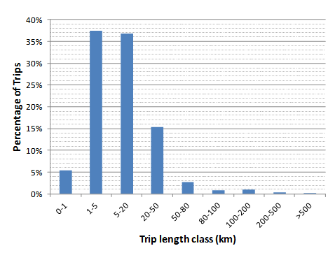 | Figure 1. Percentage of trips in each distance class for Austria[9] |
2.2. Trip Length Distribution Modelling
2.2.1. Log-normal Distribution
For range-dependent vehicles, a statistical distribution describing the probability of a certain trip length can be used to approximate the trip length behaviour. Adding the average number of trips per year yields the annual mileage allotment with respect to trip length.The statistical analysis of the trip distribution data available for 6 EU countries demonstrates a strong resemblance with the log-normal distribution, which is a typical distribution capable of describing various applications in economics. This distribution has a probability density function described as[11]: 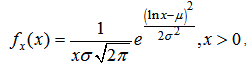 | (1) |
where X is the random variable, and μ,σ are the distribution parameters. The respective cumulative distribution function is given by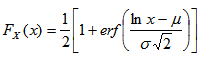 | (2) |
where erf(x) denotes the error function. The statistics of a log-normal distribution are then expressed as: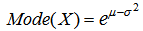 | (3) |
 | (4) |
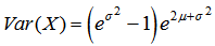 | (5) |
which represent the mode, expected value (mean) and variance of the distribution respectively. After some manipulations, it can be deduced that μ and σ can be expressed as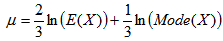 | (6) |
 | (7) |
In this way, an equivalent log-normal distribution can be constructed based on available statistical data. Moreover, these two equations require a minimum possible user input, which can be easily obtained from the actual trip distribution curves, i.e. the mean trip length that passenger cars travel and the length most commonly covered. By using the available statistical data[9], the lognormal distribution parameters were calculated. The results are presented on Table 1 for six selected countries. From the above, it can be observed that there are similarities as well as significant differences in terms of trip length characteristics. Portugal shows a distinct behaviour, since no trips were reported for distances lower than 20km. Despite this issue, it can be used as an example of the effect that totally different distributions can have upon different vehicles technologies.| Table 1. Log-normal parameters for each country |
| | Country | E[X] (km) | Mode[X] (km) | | Austria | 18 | 2.5 | | Finland | 25 | 10 | | France | 23 | 12.5 | | Netherlands | 12 | 2.5 | | Portugal | 80 | 65 | | Sweden | 30 | 10 |
|
|
An example of applying the log-normal distribution as an approximation of the trip distribution can be seen in Figure 2.  | Figure 2. Log-normal distribution approximation for trip lengths in Austria (logarithmic scale) |
In order to validate the approximation compared to the actual statistical data a comparison was carried out. By multiplying the percentage of trips in each distance class with the average distance of the respective class the total mileage was calculated. A comparison between the statistical and the approximated trip distribution for Austria can be seen in Figure 3.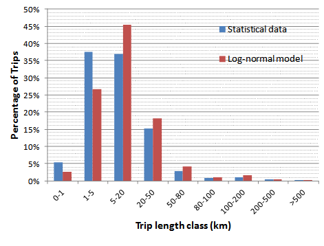 | Figure 3. Comparison of actual data with the applied log-normal distribution fit approach for Austria |
It should be noted that, in order to fully implement the mileage distribution based on the trip distribution, the average number of trips per day is also needed. These three parameters can fully accommodate a mileage distribution approximation of the available data.A comparison of all six countries in terms of the relative error (e=[data– estimation]/ data) between actual and approximated total mileage is presented on Table 2. | Table 2. Log-normal parameters for each country |
| | Country | Error (%) | | Austria | 8.79 | | Finland | 9.45 | | France | 9.07 | | Netherlands | 0.81 | | Portugal | 4.59 | | Sweden | 2.82 |
|
|
The validation showed that the proposed methodology can approximate the trip length distribution in the considered examples with acceptable accuracy, which is less than 10 % for the studied countries.
2.3. Mileage and Energy Modelling
This trip distribution approximation was developed in order to achieve a more realistic estimation of energy consumption for range-dependent vehicle technologies as opposed to the simple mileage concatenation used for conventional vehicles. In order to estimate fuel consumption, the Tier 3 method according to the EMEP/EEA Guidebook requires the combination of emission factors and activity data. The different activity data and emission factors are attributed to each driving situation as follows: 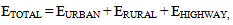 | (8) |
where E denotes the emission type of interest in each respective driving condition (urban, rural, highway). For the sake of simplicity, this paper will only focus on the hot emissions (energy consumption /CO2) part, while the evaporation effect will also be omitted. For similar reasons, the road slope is considered (flat road).Following the analysis in the previous section, if this basic concept is transformed into a continuous relation, the consumed fuel for trips with length s in (a,b] and speed v within (u,w) can be generally expressed as follows: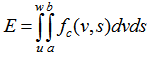 | (9) |
where fc denotes the consumption function which depends on both the average speed v and the trip length s. Thus, if a vehicle is equipped with n types of propulsion this would lead to a total annual consumption of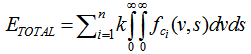 | (10) |
where k is the number of trips per year.
2.3.1. Mileage
The previous log-normal approximation of the trip distribution will be applied for the estimation of mileage: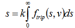 | (11) |
where s is the total mileage, k is the number of trips per year, ftrip denotes the trip distribution function with respect to a given trip length s and average trip velocity v. The average speed can be either fixed or a function of s – v(s). Initially, the speed dependency will not be considered.Using the lognormal statistics, the probability that the trip length is between a and b equals: | (12) |
or | (13) |
where erf(x) denotes the error function. In a similar fashion, the probability that the trip length is higher than c equals: | (14) |
Since the available statistical data are discrete, it would be needlessly complex to aim for a continuous solution, thus a discrete form of mileage concatenation will be employed: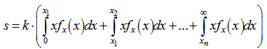 | (15) |
where n is the number of mileage bins and x1, x2, .... xn are the limits of these bins. The solution to the last term in (15) is given by[10] in the form of the partial expectation of a log-normal distribution: 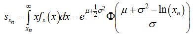 | (16) |
where Φ is the cumulative distribution of the standard normal distribution. Therefore it can also be written as: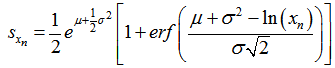 | (17) |
In order to calculate the intermediate, upper- and lower-limited, mileage bins, e.g. the (x1, x2] range, where x2>x1, the resulting mileage would become: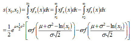 | (18) |
by invoking the previous equation (16). Thus, by establishing a discrete set of mileage bins, the mileage in each such bin can be expressed using expressions (17-18).
2.3.2. Speed Dependency
Closed-form solutions for the calculation of mileage in each mileage bin have been derived with respect to the trip distribution, which was approximated by a log-normal distribution. However, a typical energy consumption function is a linear function of the travelled distance and a coefficient dependent on the average speed. Given that, each mileage part is treated separately as a mileage bin, one would also have to provide an equivalent speed distribution. The latter one could also be dependent on the relative trip length as mentioned previously. In this approach, trip length and average speed are treated as independent variables; the average speed assigned to each distinct mileage bin is fixed for this entire mileage range. As a result, the total consumed energy for a vehicle would be: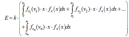 | (19) |
where fc1, fc2, ... fcn are the energy consumption functions dependent on the average speed and mileage bin of interest, rather than a continuous dependency and v1, v2,...vn are the average speed values which are distinct, yet constant for each mileage bin.
2.3.3. Other Initial Conditions
Depending on the exact nature of the vehicle powertrain, additional parameters might be necessary to consider. In electric powertrains with all-electric driving capability, for instance, the initial state charge of the battery (SoC) for each mileage bin should also be considered. This could be modelled in a way similar to the speed distribution (mileage bin dependency) in this study or in a more complex and detailed approach, bearing in mind that more complex socio-psychological models could probably be used to estimate the connection between initial charge and related trip length.
2.4. Software Implementation
2.4.1. Background
The methodology analysed in the previous paragraphs was integrated into a custom software application called SIBYL[12]. The software has a modular base, consisting of a series of virtually independent and sequential modules (Figure 4), each of them being responsible for the calculation of a certain metric (e.g. stock, mileage distribution, energy consumption etc.). It uses a bottom-up approach in forming total activity, rather than a top-down approach that would come from a demand module. Traditionally, new registrations are calculated as the difference of the size stock minus the surviving stock from the previous year. A new scenario starts by formulating the vehicle stock projection, which can be manually altered based on desired assumptions on market growth, stock growth, or vehicle utilization patterns.The average mileage combined with the previously estimated stock yields the total vehicle-kilometres. The classification of vehicles in different categories provides then the average projected mileage per technology and energy source.The calculation of activity per vehicle type in conjunction with fuel consumption and emission factors can then lead to a bottom-up energy consumption and emission estimation. The model contains emission and consumption factors for a variety of modern vehicle technologies, based on extensive powertrain software modelling and simulations of real-world driving cycles as well as actual vehicle data. Real – life vehicle characteristics were used for the development of the vehicle models and the advertised performance and fuel consumption specifications served as feedback to calibrate the results. A correlation diagram has been obtained for each such vehicle category (and fuel type for multi-fuel technologies), e.g. by simulation and testing procedures. The energy consumption factors are speed and trip-length dependent in the case of advanced powertrains. This study will focus on the trip length and mileage distribution module which incorporates the aforementioned modelling process. The implemented simulation tool also contains speed and battery state of charge distribution capabilities in order to investigate the impact of all three parameters on the emission output of selected e-mobility technologies.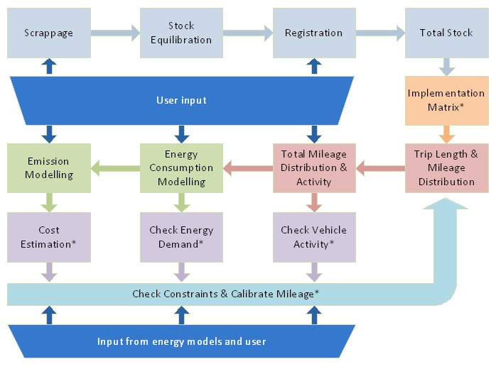 | Figure 4. Simplified SIBYL model block diagram |
3. Simulation and Results
In the following results, four vehicles have been used to demonstrate the effect of trip distribution along with speed and related initial conditions: a hybrid electric vehicle, an electric vehicle with range extender, a plug-in hybrid electric vehicle (small battery) and a medium gasoline vehicle. The latter one has been used to investigate if a detailed trip distribution can also affect conventional vehicles. The basecase simulation parameters are listed on Table 3 below. The trip distribution parameters of Austria (mean=18, mode=2.5) have been used for the log-normal distribution approximation. The speed distribution is based on the assumption that shorter trips correspond to urban driving where lower average speeds are reported and as trip distances increase, the average speed increases.| Table 3. Simulation parameters |
| | Mileage bin (km) | Speed (km/h) | Initial SoC (%) | | 0-1 | 10 | 65 | | 1-3 | 20 | 70 | | 3-10 | 30 | 75 | | 10-20 | 40 | 85 | | 20-50 | 50 | 85 | | 50-80 | 60 | 85 | | 80-100 | 70 | 85 | | 100-200 | 80 | 85 | | 200-500 | 90 | 85 | | 500- | 100 | 85 |
|
|
Figure 5 shows a comparison in terms of tailpipe average gCO2/km among the basecase, a totally different travelling pattern like Portugal (Scen2, mean=80, mode=65) and a more realistic one, Sweden (Scen1, mean=30, mode=10) and its subsequent effect on different technologies.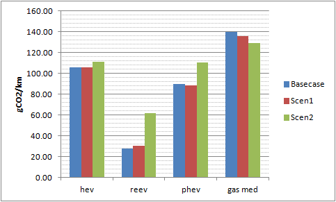 | Figure 5. Comparison of CO2 emissions of various technologies for different trip distributions |
The results are reasonable; the range extender vehicle (reev), which boasts the greatest all-electric range, shows a performance which deteriorates rapidly as the trip distribution moves outside this range. The Hybrid vehicle (hev) is only slightly affected in the extreme case (Portugal), while the plug-in hybrid (phev) shows a more complicated behaviour; CO2 emissions drop a bit for the intermediate scenario and rise significantly in the extreme case. This could be attributed to the increase of the Mode value which is close to the range of this PHEV. Finally, the conventional gasoline vehicle (gas med) indeed shows that it is affected by the different distribution patterns, mostly as a result of the varying average travelling speed with trip distance.| Table 4. CO2 emissions change compared with the basecase |
| | Vehicle | Scen1 (%) | Scen2 (%) | | hev | 0.34 | 5.17 | | reev | 9.57 | 122.41 | | phev | -1.87 | 22.83 | | gas med | -2.93 | -7.51 |
|
|
The different speed distribution (linear), as shown in Table 3, combined with majority of trips being around 50-100 km, where there is an ideal “notch” in CO2 emissions for the respective speeds, can explain the drop in CO2 emissions for the gasoline vehicle. The results are summarized in Table 4 (relative emissions compared to the basecase).In the second simulation the role of speed is investigated for the intermediate scenario (Scen1) in terms of trip distribution, following the distribution of Table 5. The relative speed increase with trip distance has been maintained, but the distribution is no longer linear. The results are shown in Figure 6. | Table 5. Simulation parameters for speed and initial SoC subscenarios |
| | Mileage bin (km) | Speed (km/h) | Initial SoC (%) | | 0-1 | 15 | 65 | | 1-3 | 15 | 65 | | 3-10 | 15 | 65 | | 10-20 | 30 | 65 | | 20-50 | 30 | 65 | | 50-80 | 30 | 65 | | 80-100 | 100 | 65 | | 100-200 | 100 | 65 | | 200-500 | 100 | 65 | | 500- | 100 | 65 |
|
|
In this case, the low speed for small distances clearly favours the hybrid drivetrains, which show a similar reception compared to the REEV and the gasoline vehicles, on which emissions increase by 25-30%. The HEV performance even appears to improve by almost 5%. This fact could be attributed to the HEV electric drivetrain optimization at very low speeds. Finally, in the last simulation run, the influence of the starting battery state of charge is investigated upon the same scenario (Scen1) as depicted in Table 5; the starting SoC remains constant for all distance classes. 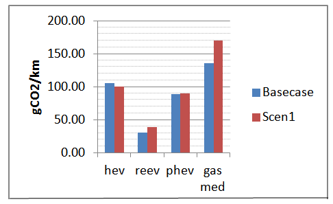 | Figure 6. Comparison of technologies when applying different speed distributions |
As expected, Figure 7 delivers the catalytic effect of the state-of-charge level on the usage of the alternative power source. The PHEV and the REEV vehicle performances deteriorate significantly as distance increases. Reasonably, the REEV is more sensitive as the low starting battery level effectively diminishes the all-electric range. 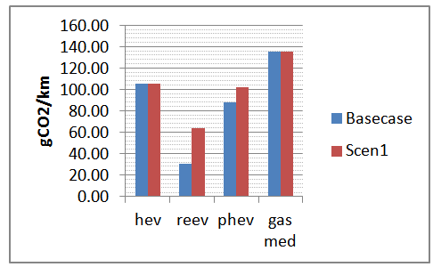 | Figure 7. Comparison of technologies when applying different initial SoC distributions |
4. Conclusions
The paper presents an attempt to model collected trip length statistical data in the form of a log-normal distribution. The resulting fit is considered satisfactory for the cases under study. This distribution is then used to form the mileage distribution, which is concatenated into discrete distance classes. Closed-form mathematical expressions are extracted by integrating each distance class. Finally, this methodology is incorporated in a thorough transport model; the tool is then used to evaluate the impact of the modelling approach on technologies which clearly depend on range resolution.The results successfully demonstrate the advantage of the proposed model in showing the true potential of electrified vehicle technologies. Moreover, further research can extend the study to include other technologies with range dependency such as bi-fuelled vehicles (e.g. gasoline – liquid petroleum gas), as well as investigate the correlation of average speed and trip length.
References
| [1] | White paper, “Roadmap to a Single European Transport Area – Towards a competitive and resource efficient transport system,” Impact Assessment, Brussels, 2011. |
| [2] | Regulation 2009/443/EC of the European Parliament and of the Council of 23 April 2009 setting emission performance standards for new passenger cars as part of the Community’s integrated approach to reduce CO2 emissions from light-duty vehicles (OJ L140, 5.6.2009, p. 5). |
| [3] | COPERT 4, v.10, 2013, Emisia, Thessaloniki, Greece.[Online]. Available:http://www.emisia.com/copert/General.html |
| [4] | EMEP/CORINAIR, Atmospheric Emission Inventory Guidebook, 3rd edition, European Environment Agency, Copenhagen, 2013.[Online]. Available:http://www.eea.europa.eu//publications/emep-eea-guidebook-2013 |
| [5] | Intergovernmental Panel on Climate Change, IPCC Guidelines for National Greenhouse Gas Inventories, Hayama, Japan, Volume 2, Energy.[Online]. Available: http://www.ipcc-nggip.iges.or.jp/public/2006gl/vol2.html |
| [6] | Adra N., André M., “Analysis of the trip length for road vehicles: statistics and trends,” Report INRETS-LTE 0429, Nov. 2004. |
| [7] | Project MESUDEMO, “Methodology for establishing general databases on transport flows and transport infrastructure networks,” Final Report, Dec. 2000 |
| [8] | Swiss Confederation and Federal Statistical Office, “Mobility and Transport, Pocket Statistics 2010,” FSO, 2010 |
| [9] | Eurostat, “Development of EU Passenger Mobility Statistics Final Report,” Dec. 2000 |
| [10] | Aitchison, J. and Brown, J.A.C. (1957), The Lognormal Distribution, Cambridge University Press. |
| [11] | Johnson, N. L., Kotz, S., Balakrishnan, N. (1994), "14: Lognormal Distributions", Continuous univariate distributions. Vol. 1, Wiley Series in Probability and Mathematical Statistics: Applied Probability and Statistics (2nd ed.), New York: John Wiley & Sons. |
| [12] | SIBYL 2.0, 2013, Emisia, Thessaloniki, Greece.[Online]. Available: http://www.emisia.com/sibyl/SIBYL.html |
 Abstract
 Reference
 Full-Text PDF
 Full-text HTML