1. Introduction

The study of the demand for money has a central role for the conduct of monetary policy. For instance, in 1994, in order to attain price stability during the financial crisis, the Central Bank of Mexico established a reserve money target based on projections on the demand for money. This policy was based on the assumption that the demand for money remained stable during the financial crisis. However, Mexico is a country that has experienced a considerable variability in inflation, interest rates and exchange rates, which could cause possible instability in the money demand function. This paper investigates whether this function remains stable during the period 1980-2005 in Mexico.

In spite of its importance for monetary policy, this issue has not usually been addressed in the relevant literature for Mexico. For example, in the study of Desentis (1997), the stability of the estimated money demand is not examined. Ramos Francia (1993) investigates the stability of the demand for M1 in Mexico, but this study extends only to 1990.

The empirical evidence on the stability for the demand function is mixed. Rogers (1992) finds that there is clear no evidence of structural stability on the estimated equation during the period 1977-1985. On the other hand, Cuthbertson and Galindo (1999) find a stable money demand function for the period 1976: IV to 1990: III.

In a more recent study, Khamis and Leone (2001), provide evidence of a long term cointegration relationship between real currency, real consumption and inflation rate, using monthly data for the period 1983:1-1997:6. Furthermore, the authors find that the dynamic model of real currency demand remained stable even after the financial crisis in 1994.

This paper investigates whether there exists a cointegration relationship between real money, a scale variable and an opportunity cost variable, using the methodology of Johansen and Juselius (1990). The scale and opportunity cost variables are measured in different ways, following Mankiw and Summers (1986). In addition, the short run money demand is estimated in error correction form, using the general to specific methodology suggested by Hendry and Richard (1982, 1983).

This paper extends the study of Khamis and Leone (2001) in several interesting ways. First, the study period includes data from 1980: I to 2005: II, which is important as we are concerned with long term relationships. Second, following the literature on this subject, this study uses quarterly rather than monthly data. This avoids the problem of repeating the same data for each month of the same quarter when monthly data are not available. Finally, this study incorporates the interest rate as a determinant of the long term money demand, which is consistent with the empirical evidence found in other countries.

The results of this study suggest the presence of a long term relationship between real money balances, consumption expenditures and interest rates. The study indicates the existence of two additional determinants of real money balances in the short run to those found in Khamis and Leone (2001): changes in private expenditures and changes in the depreciation rate. The stability tests suggest parameter constancy throughout the examined period.

This paper is organized as follows. Section II provides a description of the data. Section III presents unit root tests along with the results of the cointegration test between real money balances, consumption and interest rates. Section IV provides the estimated model in error correction form and the results of stability tests. Section V presents conclusions.

2. The Data

The data for this study are obtained from the International Financial Statistics, published by the International Monetary Fund. Following previous studies on stability of money demand, this paper uses quarterly unadjusted data. The study period is from 1980: I to 2005: II. All variables are in natural logarithms, with the exception of the interest rate.

In the literature of money demand, there is general agreement that in the long run, the level of real money balances is a function of a scale variable, such as income or wealth, and a measure on the opportunity cost of holding money, such as the interest rate, the inflation rate or the return on foreign assets.

Because of its importance for issues of monetary policy, this study concentrates on the demand for real M1 (m_t), which is defined as the sum of transferable deposits and currency outside deposit money banks. This variable is more appropriate in models that emphasize that money is used for transaction purposes.

Following the arguments given in Mankiw and Summers (1986), three different scale variables are applied, real GDP (y_t), real private consumption expenditures (pc_t) and industrial production index (ip_t). Moreover, two different interest rates are used, the one month treasury bill rate (tr_t), and the 60-day deposit rate (dr_t). Money balances and consumption expenditures are deflated by Consumption Price Index, since this variable is a better determinant of transaction balances than GDP deflator, as explained by Muscatelli and Spinelli (2000).

Following Khamis and Leone (2001), the exchange rate depreciation (dep_t) is used as a proxy variable of the return on foreign assets. Inflation (Δp_t) and depreciation rate (dep_t) are calculated as the percent change over the previous quarter, and they are annualized.

Figure 1 shows the series for real money, private consumption and interest rates. The first panel illustrates the long term relationship between real money and real consumption. The second panel shows the long term relationship between interest rates and the inverse of real money.

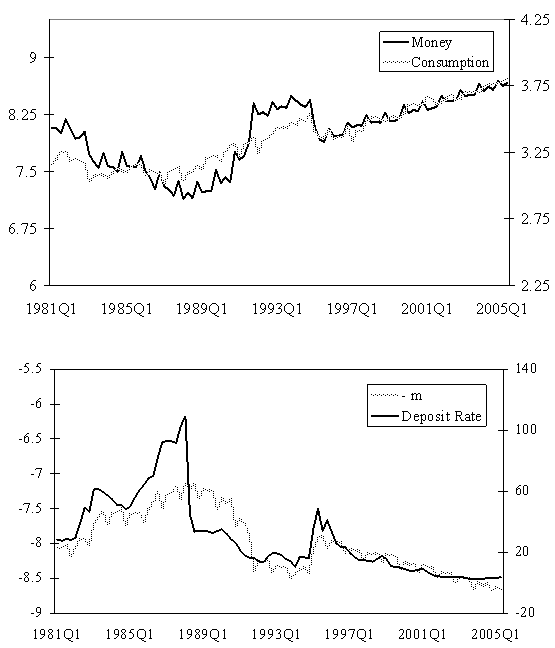Figure 1. Real Money, Real Consumption and Interest Rates

The series reflect the major macroeconomic episodes in the analyzed period. As can be seen, there is a substantial declining in real money balances and a gradual increase in the interest rates following the debt crisis in 1982. This is explained because the Mexican economy experienced a high inflation during that period. At the end of 1987, there is a stabilization period with the establishment of the Pacto. During this period, m and pc increase and dr declines gradually until the financial crisis in 1994. In general, these figures suggest the possibility of a long term relationship between m, pc and dr.

3. Long Run Behavior and Cointegration

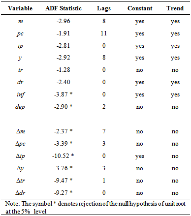
Preliminary Tests: Unit Roots

Following Johansen (1988), the cointegration test requires that the time series involved are integrated of order one, or equivalently, follow a unit root process. To determine the order of integration, Augmented Dickey Fuller (ADF) tests are used. The ADF test for the variable X_t is implemented by estimating the next regression:

(1)

where z_t are optional regressors which may include a constant term and a trend, α, β and δ are parameters to be estimated, and ε_t is the error term. The number of lags p is selected according to Schwarz Information Criterion. The result of interest of this estimation is the t-ratio for the parameter α. If the t-ratio is less than the critical value, the null hypothesis that X_t has a unit root is rejected.

The results of the unit root tests are shown in table 1. At the 5% significance level, the null hypothesis of a unit root for m_t, pc_t, ip_t, y_t, tr_t and dr_t cannot be rejected. For these variables, the results using differenced data reject the null hypothesis of a unit root. In other words, there is evidence that these variables are integrated of order one, implying that we can proceed to test for cointegration. On the other hand, the results of the ADF tests for Δp_t and dep_t suggest that these series are stationary. Therefore, these variables cannot be included in the cointegration relationship.

Table 1. Unit Root Tests

Cointegration Tests

This part examines whether there exists a long term cointegration relationship between real money balances, private consumption and interest rates. Two or more non stationary series are said to be cointegrated if there exists a linear combination of these series that is stationary. The stationary linear combination may be interpreted as a long run equilibrium relationship among the variables involved.

The Johansen (1988, 1991) methodology considers a VAR written in first differences:

(2)

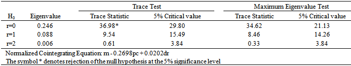
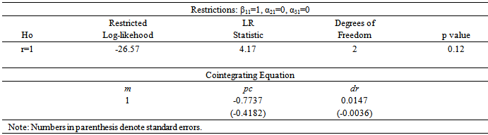
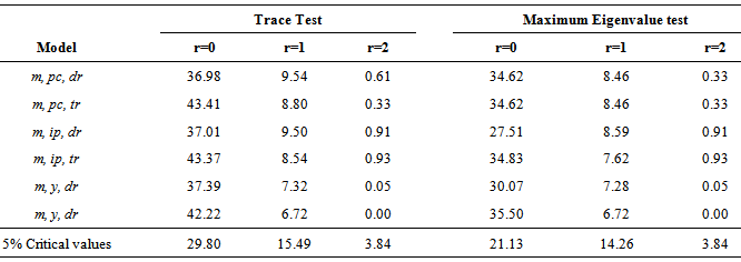
where X_t is a p vector of non stationary variables, Z_t is a vector of deterministic variables (such as seasonal dummies) and ε_t is a vector of error terms. When rank can be rewritten as where may be interpreted as a p×r matrix of cointegrating vectors and α as a p×r matrix of adjustment coefficients. Johansen (1988) estimates from an unrestricted VAR and provides a test statistic for the hypothesis that there are at most r cointegrating vectors. Then, Johansen (1991) develops tests statistics for the individual elements of the matrices α and β.

In order to determine the number of cointegrating vectors r, two types of test statistics are used, the trace statistics and the maximum eigenvalue statistics. These tests are sequentially applied for the null hypothesis of r=0 to r=p-1 until fail to reject.

Before conducting the cointegration tests, it is necessary to determine the appropriate lag length for the VAR model. To address this issue, the SIC was used. Table 2 reports the results of the cointegration tests on m_t, pc_t and dr_t, allowing for linear trends in the series, seasonal dummies, a constant in the cointegrating vector and zero lags. Both the trace and the maximum eigenvalue test suggest the presence of exactly one cointegration relationship.

Table 2. Cointegration Test

The cointegrating equation at the lower part of table 2, indicates that the elasticity of money demand with respect to consumption is approximately 0.27. The interest semi-elasticity of money demand is -0.0202. The long run interest elasticity is obtained by multiplying the semi-elasticity by the interest rate level. For the average interest rate for the study period, 29.57%, the long run elasticity becomes -0.59, which is consistent with the empirical evidence found in other countries.

Table 3 presents a test for a restricted cointegrated model, where the adjustment coefficients for pc and dr are set to zero. The restrictions are not rejected at the 5% significance level, which implies that pc and dr do not respond to the discrepancy from the long run equilibrium relationship for real money balances. In other words, pc and dr are weakly exogenous.

Table 3. Tests of cointegration restrictions

4. The Error Correction Model

Having estimated the long run money demand, the next step is to estimate a dynamic model which contains the short run adjustment to the deviation from the long run equilibrium. In the last section, it was found that the variables pc and dr are weakly exogenous. Therefore, following Hendry (1995), the short run money demand can be estimated by using a general autoregressive distributive lag (ADL) model. This methodology starts by estimating the next general dynamic specification:

(3)

where c is a constant, X_t is a vector containing pc_t, dr_t, dep_t, and Δp_t, EC denotes error correction term and D_i are dummy variables for quarter i. Following the general to specific methodology suggested by Hendry (1995), the equation above is successively estimated, excluding the variables with the lowest t-values, until a parsimonious representation is found. The resulting equation from this procedure is:

(4)

R² = 0.84S.E. = 0.057DW = 1.98

AR F(4,83) = 1.52 [0.20] ARCH F(4,83) = 1.19 [0.32]HET χ²(2) = 10.8 [0.63]

RAM F(1,86) = 0.067 [0.80]NORM χ²(2) = 205.81 [0.00]

where s.d. denotes seasonal dummies (not reported here). Numbers on parenthesis below each parameter denote standard errors. Numbers between brackets denote p values. All the parameters have the expected sign. The statistical properties if the residuals indicate the nonexistence of serial correlation, heteroskedasticity and ARCH. In addition, the Ramsey test suggests that the model is well specified. Although the normality of residuals is not supported by the Jarque Bera test, this fact seems to be due to the presence of one outlier in 1992.

The equation above has an interesting economic interpretation. In the short run, economic agents adjust their money balances by 8.6% of the deviation from the long run equilibrium in the last period. Two additional determinants of real money balances in the short run to those provided in Khamis and Leone (2001) are found, changes in private expenditures and changes in the depreciation rate. Furthermore, this equation indicates that agents respond immediately to changes in the interest rate, but the response to changes in the depreciation rate and consumption expenditures occurs after one period.

The short run elasticity with respect to the depreciation rate may be obtained by multiplying the semi-elasticity shown above by the level of depreciation rate. For the average depreciation rate on the analyzed period, which is 6.6%, the elasticity is approximately -0.00087. Although this elasticity appears low, the response of money balances becomes important with the large changes in the depreciation rate that have occurred during financial crisis. It is worth mentioning that changes in inflation rate do not seem to have an effect on the short run money balances. The estimated parameters on the seasonal dummies suggest an important increase in the demand for money during the last quarter of each year.

When the model is estimated using different scale and opportunity cost variables, the determinants of short run money balances appear to be the same. For instance, when ip is used as scale variable (after testing for cointegration and weak exogeneity), the estimation result becomes:

(5)

Again all the parameters have the expected sign, and the estimated coefficients are similar, providing robustness to the results found above.

Stability tests

Figure 2 shows the residuals of the short run money demand estimation. As can be seen in the figure, only a few residuals are outside of the two standard error bands. Figure 3 presents the series of recursive coefficient estimates along with the corresponding two standard error bands. The figure suggests that parameters become more stable and the standard errors tend to decrease as more data are employed in the estimation.

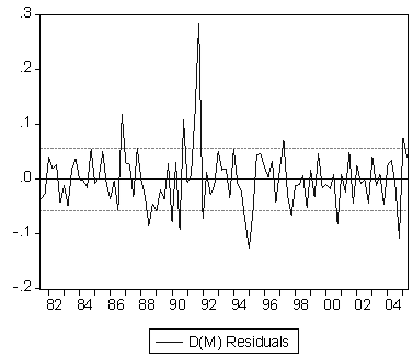Figure 2. Residuals of the Error Correction Model

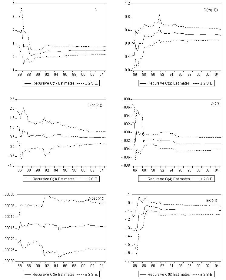Figure 3. Recursive Coefficient Estimates

The CUSUM and CUSUM of Squares tests of stability, which are based on the cumulative sum of one step ahead forecast errors, are shown in figure 4. Since the cumulative sum of recursive residuals and the cumulative sum of squares lie inside the area of the two critical lines, these tests suggest parameter stability throughout the examined period.

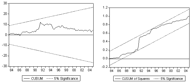Figure 4. CUSUM and CUSUM of Squares Tests

Parameter stability is also supported by the one step residuals test, shown in figure 5. With the exception of five observations, all forecast errors lie in the two standard error critical line. Moreover, a Chow forecast test for the period 1994Q4-1995Q5 (shown in Table 4) cannot reject the null hypothesis of parameter constancy during the financial crisis. In general, the stability tests suggest that the estimated parameters remained constant throughout the analyzed period.

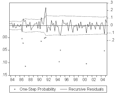Figure 5. One Step Residuals Test

Table 4. Chow Forecast Test: 1994Q4 to 2005Q4

5. Conclusions

This paper examines the demand for narrow money in Mexico for the period 1980-2005, extending the study by Khamis and Leone (2001). The cointegration tests results suggest the existence of a long term relationship between real money balances, consumption expenditures and interest rates.

The estimated error correction model indicates the existence of two additional determinants of real money balances in the short run to those found in Khamis and Leone (2001): changes in private expenditures and changes in the depreciation rate. Monetary authorities should take these variables into account for making projections on money demand.

The stability tests suggest parameter constancy throughout the examined period, despite the fact that Mexico has experienced important periods of crisis, substantial variability in inflation, exchange rates and interest rates.

Appendix

Table 5. Cointegration tests on different specifications

Table 6. Normalized Coefficient Estimates

Notes

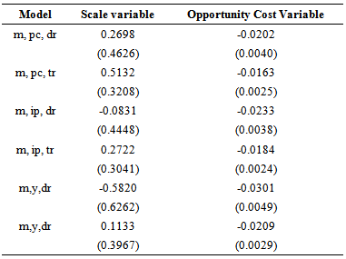
1. I thank Dennis Jansen for valuable comments. The views on this paper correspond to the author and do not necessarily reflect those of Banco de Mexico.

2. See for example Hoffman et al (1995).

3. For instance, in a study on stability of money demand in Germany, Lütkepohl et al (1999), illustrate the importance of using seasonally unadjusted data when seasonal changes may be a source of instability.

4. The return on foreign assets equals the sum of the foreign interest rate plus the exchange rate depreciation rate. Following Khamis and Leone (2001), movements in the return on foreign assets are dominated by the exchange rate changes.

5. It’s important to notice that the t-ratio test doesn’t follow the usual t distribution; critical values are tabulated from Monte Carlo distributions in Mac Kinnon (1996).

6. For the variable pc_t, the null hypothesis of a unit root is rejected at the 5% significance level when the number of lags is selected according to SIC. However, when this number is selected according to the Akaike Information Criterion, the null hypothesis is not rejected. In what follows, this variable is assumed to be I(1).

7. Seasonal dummy variables are centered (orthogonalized). Johansen (1995) argues that using centered seasonal dummies avoids the problem of affecting the trend of the level series when standard dummies are applied.

8. The cointegration test is also examined including ip_t and y_t as scale variable, and tr_t as an opportunity cost measure. However, in two cases the sign of the coefficient on the scale variable is not as expected. For comparison purposes, the results for these tests are given in the appendix.

9. For example, Hoffman and Rasche (1991), using US data from 1953 to 1988, find a short term interest elasticity in the -0.4 to -0.6 range.

10. Cuthbertson and Galindo (1999), explain that the delayed response to changes in exchange rates may occur because the exchange rate tends to move in the same direction during crisis periods, and it is generally stable during in intervening periods. Therefore, agents respond to the lagged exchange rate as the can anticipate the trend of exchange rate in the short run.