1. Introduction

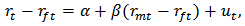
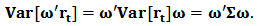
In the analysis of financial data we often have to implement regression analysis from historical data, the aim being to predict future values of the variables. In this paper we will work mainly with regression techniques applied to portfolio prediction. Classical applications are Markowitz portfolio optimization, Marcowitz (1952), and the Capital Asset Pricing Model (CAPM), developed by many leading economists in the sixties.

CAPM is a very used method for estimating the expected return of a portfolio and evaluation of risks. It is a one-factor model:

with , where is the rate of return, is the risk-free rate, is the rate of return of the market and is a random error. Typically the model is fitted by ordinary least squares (OLS).

We can put CAPM in the context of the standard linear model:

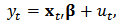(1)

with and following a density . It is useful to write the model in matrix notation:

(2)

where and are vectors and is a matrix.

In spite of well-known shortcomings, CAPM continues tobe an important and widely used model. From a statistical point of view, it is known that standard OLS estimation of presents several drawbacks. In particular many authors have pointed out its high sensitivity in the presence of outliers and its loss of efficiency in the presence of small deviations from the normality assumption, see, for instance, the books by Huber (1981), Hampel et al.(1986) and Huber and Ronchetti (2009).

Robust statistics was developed to cope with the problem arising from the approximate nature of standard parametric models. Indeed robust statistics deals with deviations from the stochastic assumptions on the model and develops statistical procedures which are still reliable and reasonably efficient in a small neighborhood of the model. In particular, several well known robust regression estimators were proposed in the finance literature as alternatives to OLS to estimate . This issue was already studied by one of the creators of the CAPM, Sharpe (1971). He suggested to use least absolute deviations (-estimator) instead of OLS (-estimator). Chan and Lakonishok (1992) used regression quantiles, linear combinations of regression quantiles, and trimmed regression quantiles. Martin and Simin (2003) proposed to estimate using redescending M-estimators.

These robust estimators produce values of which are more reliable than those obtained by OLS in that they reflect the majority of the historical data and they are not influenced by outlying returns. In fact, robust estimators downweight abnormal observations by means of weights which are computed from the data. Following the discussion in Genton and Ronchetti (2008), robustness is important if the main goal of the analysis is to reflect the structure of the underlying process as revealed by the bulk of the data, but a familiar criticism of this approach in finance is that 'abnormal returns are the important observations', and it has some foundation from the point of view of prediction. Indeed if abnormal returns are not errors but legitimate outlying observations, they will likely appear again in the future and downweighting them by using robust estimators will potentially result in a bias in the prediction of . On the other hand, it is true that OLS will produce in this case unbiased estimators of but this is achieved by paying a potentially important price of a large variability in the prediction. Therefore, we are in a typical situation of a trade-off between bias and variance and we can improve upon a simple use of either OLS or a robust estimator. This motivates the use of some form of shrinkage from the robust estimator toward OLS to achieve the minimization of the mean squared error.

That discussion on CAPM and in least-squares regression model can also be extrapolated to other models in finance based on analog statistical principles. The topic which interests us here is portfolio optimization, mainly from the point of view of prediction. The goal of portfolio optimization is to find weights , which represent the percentage of capital to be invested in each asset, and to obtain an expected return with a minimum risk. Brodie et al. (2007) presented a way to express the optimization problem as a multiple regression with constraints. It is therefore possible to perform this regression using robust methods, e.g. M-estimators, least trimmed squares (LTS) or others.

Consider a portfolio with assets and historical returns forming the rows of a matrix . For an expected return we can solve the following optimization problem: 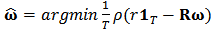with constraints and where is a penalizing function such as squaring for the OLS estimator or the Huber's function for the robust M-estimator. We use robust estimations and we solve the optimization problem to obtain a robust estimation for the portfolio weights . We then use a shrinkage estimator, see Eq. (24), to 'shrink' towards the OLS estimator and find an optimal value of the shrinkage parameter for the measures of predictive power considered in Section 4 of Genton and Ronchetti (2008).

We use Monte-Carlo simulations to study the behavior of the optimum values of for outlying returns generated by contamination or long-tailed skew-symmetric laws. The simulations give us empirical heuristics for actual applications in robust asset allocation. We consider specially the flexibility of skew-symmetric distributions and study these type of distributions which allow to model return distributions with significant skewness and high kurtosis as is usually the case of hedge funds (see for instance Popova et al. (2003)).

From a practical point of view, we implement the methods in the statistical software R. Some tools are already implemented (e.g. MCD estimator) but we have to program some other routines (constrained robust regression, multivariate shrinkage). Depending on the amount of data to be analyzed, execution can be expensive in time, consequently we have to take care about efficiency of the routines mainly if we want to apply Monte Carlo simulations using resampling methods.

This paper could be considered as an application in portfolio optimization of the skrinkage estimators studied in Genton and Ronchetti (2008). They only treat the case of estimating beta in CAPM. That estimator have been generalized to multidimensional variables need in portfolio statistical analysis. Gramacy et al. (2008) use specific shrinkage estimators (LASSO and rigde regression) in finance to estimate covariances between many assets with histories of highly variable length (missing data) but they do not the deal with robustness. That work have been developed and extended in Gramacy and Pantaleo (2010), where they consider a Bayesian hierarchical formulation, considering heavy-tailed errors and accounting for estimation risk.

The introduction to robust techniques to portfolio optimization is relatively recent compared with the Markowitz foundational paper. Nevertheless the subject have become very active in the last decade. We can mention the works of Vaz-de Melo and Camara (2003), Perret-Gentil and Victoria-Feser (2004), and Welsch and Zhou (2007). All three papers compute the robust portfolio policies in two steps. First, they compute a robust estimate of the covariance matrix of asset returns. Second, they solve the minimum-variance problem where the covariance matrix is replaced by its robust estimate. Recently, Demiguel and Nogales (2009) proposed solving a single nonlinear program, where portfolio optimization and robust estimation are performed in one step. They performed a theoretical study for M-estimators and S-estimators, in addition to a simulation using a mixture of a normal and a deviation distribution. A very recent work of Demiguel et al. (2013) have also implemented a shrinkage strategy both using shrinkage estimators of the moments of asset returns (shrinkage moments), and using shrinkage portfolios obtained by shrinking the portfolio weights directly. We have to remark that in that paper, they use shrinkage by means of a convex combination from the sample estimator (low bias), towards the target estimator (low variance). They use two calibration criteria: the expected quadratic loss minimization criterion, and the Sharpe ratio maximization criterion. We distinguish our work by the fact that use explicitly use a M-estimator as the target of the shrinkage, which enables us to use a more specific shrinkage estimator (from Genton and Ronchetti (2008)) with the calibration parameter is related to Huber's function. In fact varying that parameter allow the shrinkage model to interpolate within the family of robust estimators, the OLS estimator being a limit case for a big value of the parameter (in fact the OLS is the limit for , see Section 4). This is an advantage of our shrinkage strategy compared to convex combination of estimators. Other characteristic of our work is that use use many measures of predictive errors aside the expected quadratic loss. This is specially because in our simulated study we are interested in long-tailed and asymmetric distributions. Other reference which uses skew-symmetric laws as in portfolio optimization is Hu and Kercheval (2010) but they do not involve with shrinkage strategies.

The paper is organized as follows, in Section 2 we explain some basic issues concerning the appearance of asymmetric and long-tailed errors and robust regression, then in Section 3 we derive the robust constrained regression model associated to portfolio allocation, in particular we have a closed formula for the shift of the estimator of the parameter vector of the linear model due to linear constraints, see. Eq. 14. In section 4, we present a shrinkage robust estimator and combine it with the constrained robust regression in a procedure for the application in portfolio optimization. Section 5 illustrates the results of the combined procedure using Monte Carlo simulation, first in an ideal standard linear model and then to simulated distributions from contaminated normal and asymmetric-long-tailed laws. Finally Section 7 presents some conclusions of our study.

2. Non-normal Errors and Robust Regression

Robust statistics is an extension of classical statistics in that it takes into account the possibility of contaminated data or more generally of model misspecification. This theory was firstly developed by Huber (1964) and Hampel (1968).

There are many ways to model errors with outlier. For instance we can consider a mixture of a normal distribution with a large-variance distribution . Let be a number representing the proportion of contamination and define the neighborhood of the parametric distribution to be the set:

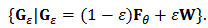(3)

can be considered as a mixed distribution between and the contamination distribution . An estimator is said robust if it remains stable in a neighborhood of . Often in theoretical studies is a multivariate normal distribution in dimension : .

In standard linear regression theory, least-squares estimator for the parameter is known to be non-robust. In section 3 we will use M-estimators to find robust estimates of parameters in portfolio allocation. In the context of the linear model (1), the general M-estimators minimize the objective function:

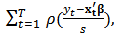(4)

with respect to and the loss function gives the contribution of each residual to the objective function. is a scale parameter. Generalizing least-squares minimization, a reasonable should have the following properties:

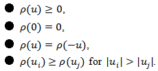For example, for least-squares estimation we have .

Let denote the derivative of . In this paper we will work with the Huber objective function and its derivative which is called Huber function and is defined by . The tuning constant controls the level of robustness. If then , which corresponds to least-squares estimation.

Differentiating the objective function (4) with respect to gives the following estimating equations:

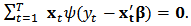(5)

Define the weight function , and denote . Then the estimating equation (5) can be written as:

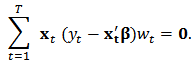Note that solving these estimating equations can be seen as a weighted least-squares minimization problem with objective function:

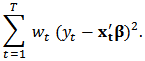The weights , however, depend upon the residuals, the residuals depend upon the estimated coefficients, and the estimated coefficients depend upon the weights. An iterative solution is therefore required. More details about M-estimators can be found in references, for instance Hampel et al. (1986).

At the end of the procedure we obtain the weights which can be collected in a diagonal matrix and then we can calculate the M-estimator in matrix notation:

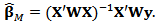
2.1. Resistant Regression (LTS)

There are other robust techniques of estimation in order to reduce the influence of outliers on the fit of a model. Following the schema of Genton and Ronchetti (2008), we will use the least trimmed squares (LTS) regression.

LTS was proposed by Rousseeuw (1985) as another robust alternative to OLS. Let us consider a linear regression model (1). The LTS estimator is defined as:

where represents the -th order statistics of squared residuals with .

The trimming constant has to satisfy . This constant determines the robustness level of the LTS estimator, since the definition implies that observations with the largest residuals do not have a direct influence on the estimator. The LTS robustness is the lowest for , which corresponds to the least-squares estimator.

2.2. Asymmetric and Long-tailed Errors

Often returns in portfolio optimization do not follow a normal distribution and the empirical distribution presents asymmetry and thick tails. In those cases we can propose errors following more flexible laws such as skew-symmetric distributions.

Skew-symmetric distributions were explicitly introduced in the literature by Azzalini (1985) with the aim to model departure from normality. Afterwards many generalizations have been introduced and it is nowadays a well studied topic because of its flexibility and theoretical tractability. We can mention the multivariate skew normal distribution studied by Azzalini and Dalla Valle (1996) and the multivariate skew distribution studied in Azzalini and Capitanio (2003). Here we will only define notations.

2.2.1. The Multivariate Skew-normal Distribution

Given a full-rank covariance matrix define , let be the corresponding correlation matrix and define vectors , . A -dimensional random variable is said to follow a skew-normal distribution if its density function at is given by:

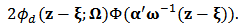where is the -dimensional normal density at with covariance matrix and is the distribution function.

We will then write and call the location, dispersion and the shape or skewness parameters, respectively. If we define a new shape parameter:

then we can write the expressions of mean vector and covariance matrix:

2.2.2. The Multivariate Skew-t Distribution

In dimension 1, standard t distribution have thick tails and then it allows to model large outliers. In the multivariate case, consider random variables , independent of , and the constant vector . We define the skew-t distribution as the one corresponding to the transformation:

(6)

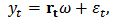
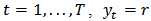
We shall write . The parameter corresponds to the degrees of freedom. A small value of will allow the presence of large outliers and when then converges to a skew-normal variable.

The density function and other formulas and properties can be found in Azzalini and Capitanio (2003). Figures 1 and 2 shows two scatterplots of a 4-dimensional skew-normal variable and skew-t variable. In section 6 we will perform simulations using these distributions in the context of portfolio optimization.

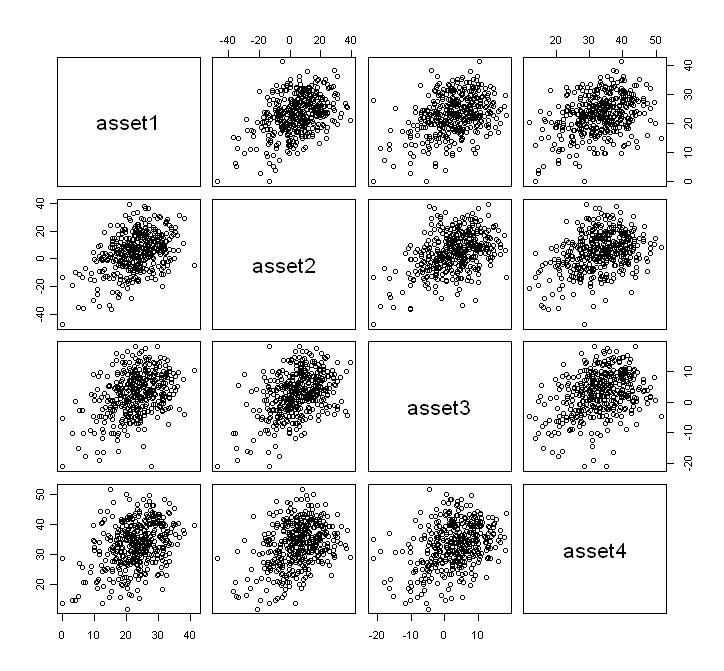Figure 1. Scatterplot of a distribution

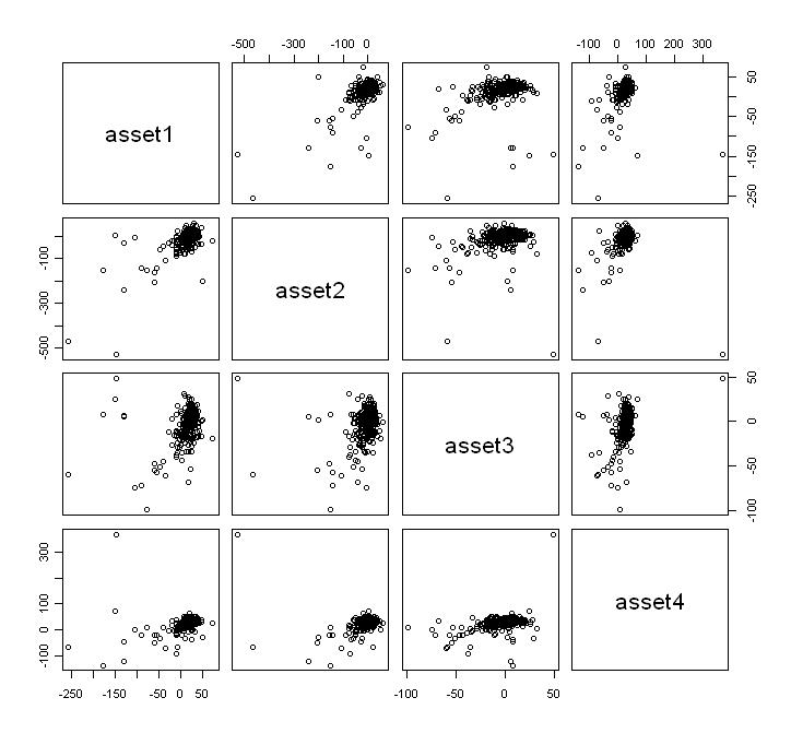Figure 2. Scatterplot of a distribution

3. Portfolio Asset Allocation

We consider assets and denote their returns at time by and denote by the vector of returns at time . We assume that follows a multivariate distribution with and .

A portfolio is defined to be a list of weights for the assets that represent the amount of capital to be invested in each asset. We assume that which means that capital is fully invested and denote the vector of weights.

For a given portfolio , the expected return and variance are respectively given by:

(7)

(8)

Following the standard Markowitz portfolio optimization procedure, we seek a portfolio which has minimal variance for a given expected return . We can express the problem as:

with constraints

(9)

(10)

where is the vector in which every entry is equal to 1.

We can find in Brodie et al.(2007) a way to model the optimization problem using a multivariate constrained regression. Here we develop details of the derivation.

We have and we can write:

In fact and are scalars and using (7) we can write the last expression as:

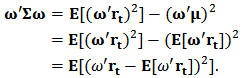Finally using (7) and the constraint (9) we have:

(11)

For the empirical implementation, we replace expectations by sample average. We set and define to be the matrix of which the row is .

The empirical version of expression (11) is:

where, for a vector in , we use the 2-norm notation: .

In summary, we seek to solve the new following optimization problem:

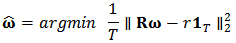with constraints

(12)

(13)

We can view this as a multiple constrained regression for the model:

for each , and with the same constraints (12) and (13).

In the optic of robustness we replace the 2-norm by a loss function which grows slower, obtaining then the problem:

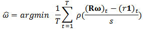with constraints (12) and (13). As before is a scale parameter which should be estimated robustly.

We have seen in the last section that the non-constrained M-estimator is: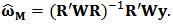

The constrained minimization is solved using Lagrange multipliers. We present the derivation in the next subsection 3.1. In the presence of independent linear constrains we obtain the constrained M-estimator :

(14)

We observe that the constrained M-estimator differs from the unconstrained by a function of the quantity .

For our problem, the constraint matrices are:

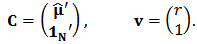(15)

3.1. Constrained Robust Regression

Using the notation of weighted least-squares regression and in the presence of`the linear constrains , we can write the Lagrangian:

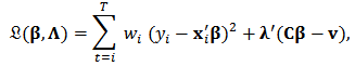where is a vector of lagrange multipliers, is a matrix and is a vector.

In matrix notation:

Differentiation with respect to and gives the equations:

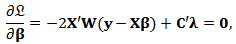
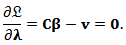From the first equation we find:

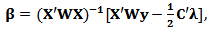(16)

and replacing this into the second equation we get:

(17)

From this, we obtain the value of :

(18)

and replacing this into expression (16) we find the expression of the constrained estimator:

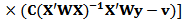Recall the formula of the non-constrained weighted estimator:

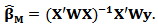Using this the final expression of the constrained M-estimator can be written:

(19)

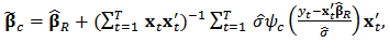
4. Shrinkage Robust Estimator

Genton and Ronchetti (2008) have defined a robust estimator with shrinkage for the linear model:

(20)

where is a robust estimator of , is a robust estimator of scale such as the median absolute deviation (MAD), and is the Huber's function. As we have seen in Section 2, there are many proposals for the robust estimator , see for instance Hampel et al. (1986).

The tuning constant allows us to control the level of shrinkage. If we find the robust estimator and if we find the least-squares estimator (OLS).

Indeed, in then for all values of then the rightmost expression in (20) is zero and we have , the robust estimator. On the other side, if then and equation (20) simplifies to:

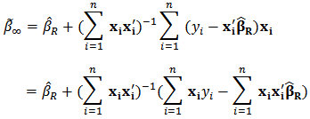Distributing the expression and recognizing the expression of ordinary least-squares estimator we obtain:

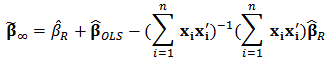The rightmost expression simplifies and we obtain the limit expression:

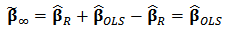(21)

As was discussed in the Section 1, if the goal of modeling is to find a model which reflects the bulk of the data then the robust estimation is the most adequate method because outliers are under-weighted. Nevertheless from a predictive point of view, outliers in finance could be considered as interesting data. So it is important to study if, by varying the constant , we can improve the predictive power with respect to least-squares or robust estimators.

There are many choices for measuring the quality of the prediction. For normal-distributed errors, the most used criterium is the mean squared error (MSE). However for asymmetric or long-tailed distributions there is not a standard choice.

Following Genton and Ronchetti (2008) we consider a family of measures:

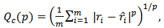(22)

where is the shrinkage constant used to estimate the expected returns . The case give us the MSE measure. We will be interested in , and .

An important tool to compare the shrinkage estimators is the relative gain:

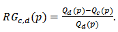(23)

It will be useful to analyze if shrinkage with a level offers more predictive power than the robust estimator or the OLS estimator .

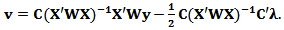
4.1. Application to Portfolio Optimization

In classical portfolio optimization the first stage in general is to estimate the mean and the covariances . We can use the historical data and use robust methods to obtain (robust) estimators and , as explained by Welsch and Zhou (2007). Some methods such as minimum covariance determinant MCD or FAST-MCD are already implemented in statistical software such as R.

We have seen in section 3 how to write the classical portfolio optimization problem as a multivariate constrained regression problem and then we considered the robust setting of the problem. In this formulation, we need only a robust estimator of which enters into de constrains matrix (see formula (15)). We will use the MCD estimator which is already implemented in R.

In subsection 3.1 we have found the formula of the robust constrained estimator of the portfolio weights. We can now try to apply the shrinkage to but then the constraints are no more satisfied. We need to use equation (19) one more time but for this we have to recalculate the matrix .

To be precise we present next a detailed description of the procedure step by step.

1. Calculate robust estimator and the regression matrix of weights . This can be do with standard routines of statistical software such as R.

2. Use to obtain the constrained estimator given by formula

3. Let be de tuning constant of shrinkage then calculate the shrinkage estimator:

(24)

4. Using , calculate the new weight matrix associated with this estimator. We need to calculate standardized residuals 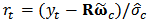, where is a robust estimate of scale of the residuals. The matrix is diagonal with -th component:

5. Use to obtain the shrinkage constrained estimator given by formula

We will use Monte-Carlo simulations to study the behavior of the optimum values of with respect to the different prediction error measures (values of in (22)) for normal and outlying returns generated by contamination (mixture) and by skew-symmetric laws.

A suitable shrinkage could vary in time depending on new available historical data. Anyway at any moment the Monte Carlo simulation can be performed to assess an optimum value of this shrinkage parameter for future estimations of the portfolio weights.

We remark that the computation complexity of this procedure depends of the actual implementation of the robust estimation and the matrix operations involved. Supposing that Iteratively Reweighed Least Squares is used in step 1. and only a few iterations are sufficient for convergence, the number of operations involved in all the steps is of the order 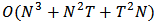. Taking N (the number of the assets) fixed, the computational complexity becomes . In consequence, even if it is possible to assess efficiency of Monte Carlo simulation by changing , the computational work increases too, as well as the collateral computational errors. A better study of this remains to be done.

5. Monte Carlo Simulations

In this section we perform simulations based on the paper of Genton and Ronchetti (2008) but in the multivariate case. We will apply the general strategy to portfolio optimization in section 6. We consider the linear model:

with a vector, i.i.d. errors and a multivariate normal. As the first example we consider two covariates:

and we take the values , , , with independent variables.

We take and include of outliers (contamination) for and from .

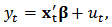
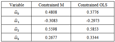
We use M and LTS estimators, and , to obtain robust estimates of . The estimated values are:

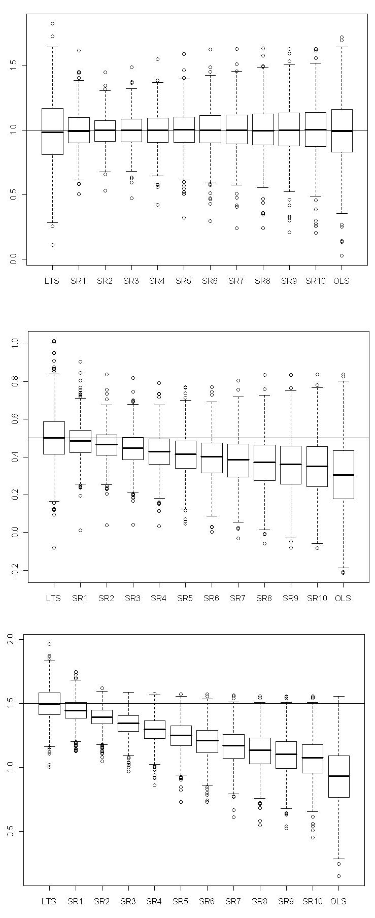
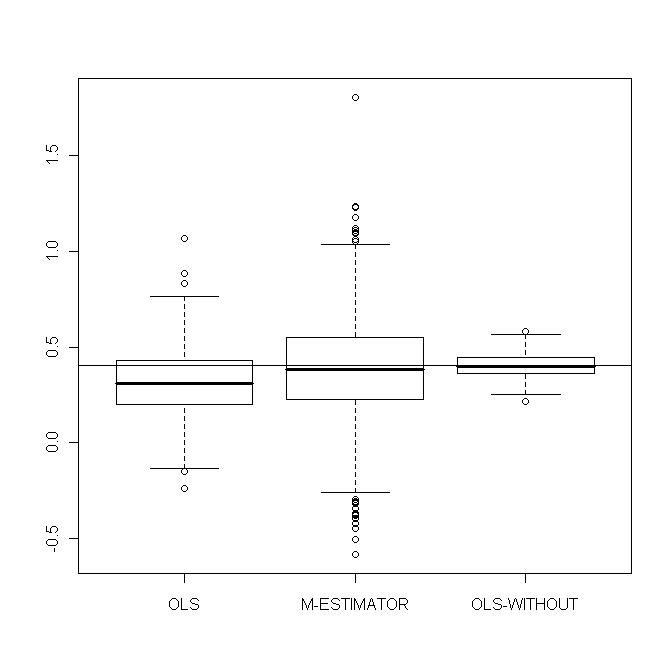
We observe that the OLS estimates are biased and will not be useful for future predictions. We can now use the shrinkage robust estimator (called in the sequel), , of with shrinkage constant . In order to analyze the effect of outliers, we simulate 1000 training data sets of size each and containing outliers as indicated. For each sample we estimate by LTS, OLS and with . Figures 4 show boxplots of these estimates over the 1000 simulated training data.

The LTS estimators of and have smaller bias than OLS estimators. We observe that for some values of , the variance of is reduced at the cost of a small increase in bias.

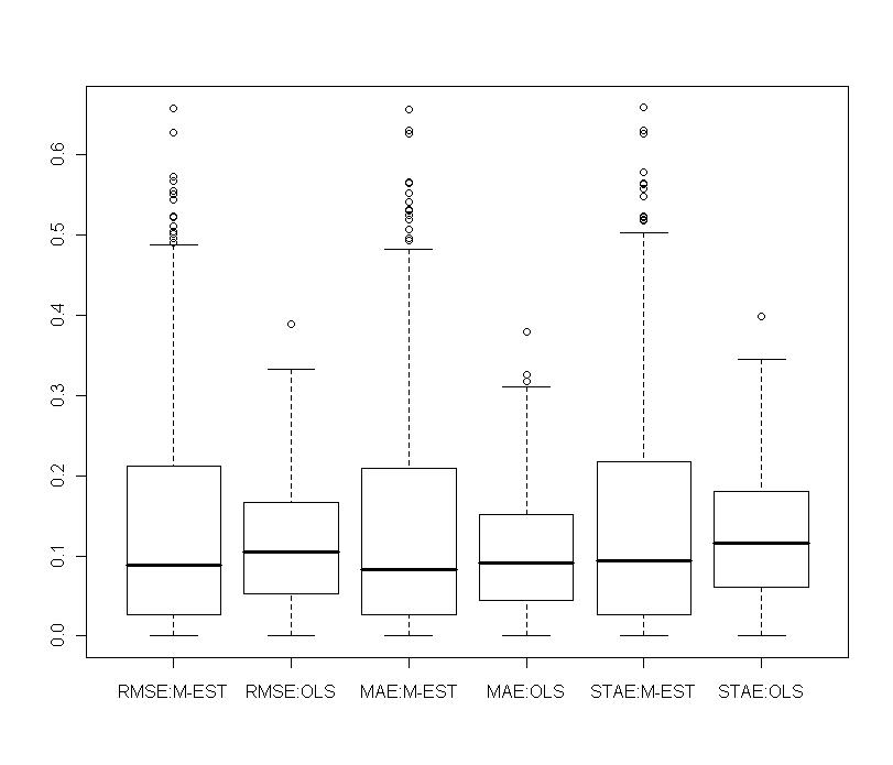
Next we investigate the effect of outliers and shrinkage on the prediction of future observations. More precisely, for each of the 1000 estimates , we compute the predicted values .

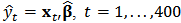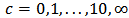
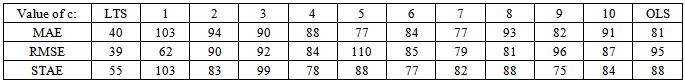
We consider the measures of quality of prediction with the shrinkage robust estimator , defined in (22) with three choices for . For we have the root mean square error (RMSE), for the mean absolute error (MAE) and for the square root absolute error (STAE).

In Table 1 we report the frequencies of selection of a minimum measure of prediction for a range of values of 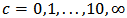over the replicates. As can be seen, the optimal which minimizes a certain measure of quality of prediction is not exclusively concentrated at the 'limit' estimators LTS and OLS. The RMSE measure is related with least squares estimation, consequently OLS is selected most of times. We observe that a shrinkage constant of is optimal for MAE and is optimal for STAE. If we are interested in a more precise value of the constant , it is possible to refine the search around the values 2 or 3 of the parameter and use a smaller step size.

Table 1. Normal contamination: frequencies of selection of a minimum measure of prediction

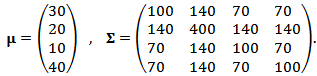
We have defined the relative gain by in (23). Denote by the value of minimizing for a fixed . Figure 3 depicts boxplots over the 1000 replicates of and for and 2, that is, the relative gain compared to LTS and OLS estimators using STAE, MAE and RMSE respectively.

We remark that in terms RMSE, the gains of compared to OLS are small. In terms of MAE and STAE, the gains can reach . The gains compared to LTS go rather in the other direction.

Figure 3. Normal contamination: relative gains obtained with shrinkage robust estimators compared to LTS and OLS on various measures of prediction (RMSE, MAE, STAE)

Figure 4. Normal contamination: boxplots of and for several values of the shrinkage constant

6. Application to Portfolio Optimization

Monte Carlo simulations can give us empirical heuristics for actual applications of the shrinkage robust asset allocation. We have already mentioned the flexibility of skew-symmetric distributions and we will especially study these types of distributions which allow to model return distributions which have significant skewness and high kurtosis such as hedge funds (see for instance Popova et al. (2003)). In this paper we will perform only a empirical study.

6.1. Normal Data with Normal Contamination

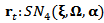
We consider a portfolio of assets. In this example, we suppose that returns are generated from a 4-dimensional normal distribution

(25)

with parameters:

(26)

We will include of contamination from where:

(27)

We interpret this as independent returns with large variance. We used a general scaling constant of 10 and this explains the order of magnitude of mean vectors and variance matrices.

Recall that in portfolio optimization, the regression equation is:

(28)

the expected return of the portfolio and with constraints (12) and (13).

We simulate a contaminated test sample of size and take . In practice we don't know the theoretical mean vector and we only have the matrix of all returns. As long as we have outliers we need a robust estimate of denoted . This can be performed using the method called "fast MCD" developed by Rousseeuw and Van Driessen (1999) which is more general and compute a robust covariance matrix estimator too. The robust estimate of is:

(29)

In Figures 5-8 we simulate 500 data sets of size 400 each and compare the M-estimates and OLS estimates of contaminated data with the OLS estimates of non-contaminated data. The bias is much smaller for the M-estimates but for some variables it is not null. Anyway in this paper we worked with M-estimators because we could find analytical formulas for constrained regression (Section 3.1). These formulas allowed us to implement shrinkage and to verify the constraints. There is also the possibility to use more resistant estimators but in that case it is necessary to use others methods to project the shrinked weights onto de constrained subspace.

Figure 5. OLS-estimates, M-estimates and non-contaminated OLS estimates of

Figure 6. OLS-estimates, M-estimates and non-contaminated OLS estimates of

Figure 7. OLS-estimates, M-estimates and non-contaminated OLS estimates of

Figure 8. OLS-estimates, M-estimates and non-contaminated OLS estimates of

Following the algorithm described in subsection 4.1 we will use M-estimator as initial robust estimate. The estimates are:

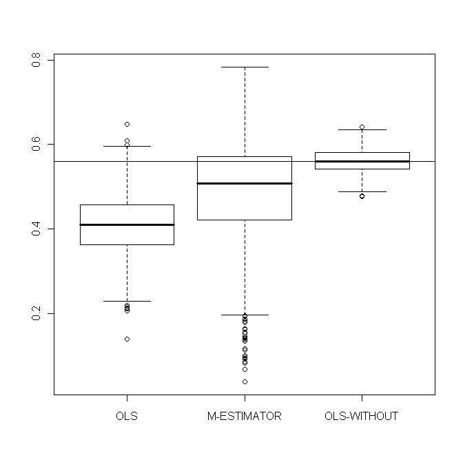
As these values are computed using constraints, it is difficult to assess the standard errors and intervals of confidence analytically. The Monte Carlo simulations will show that the interquartile ranges (IQR) are large and this reflects the instability of classical portfolio optimization.

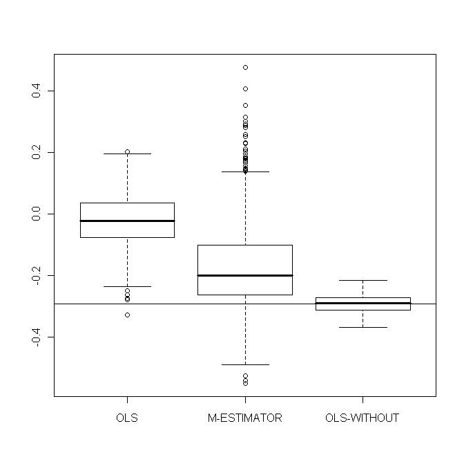
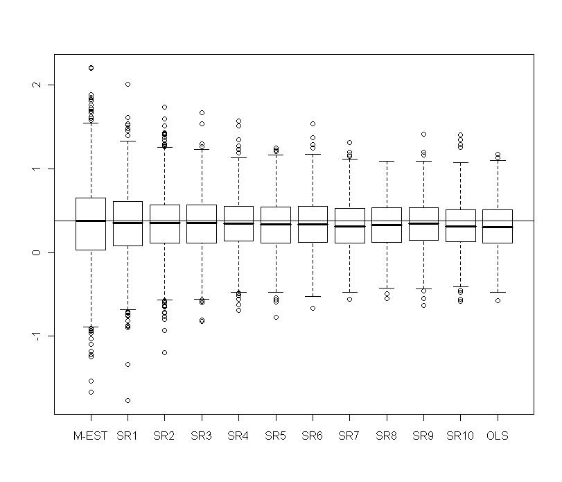
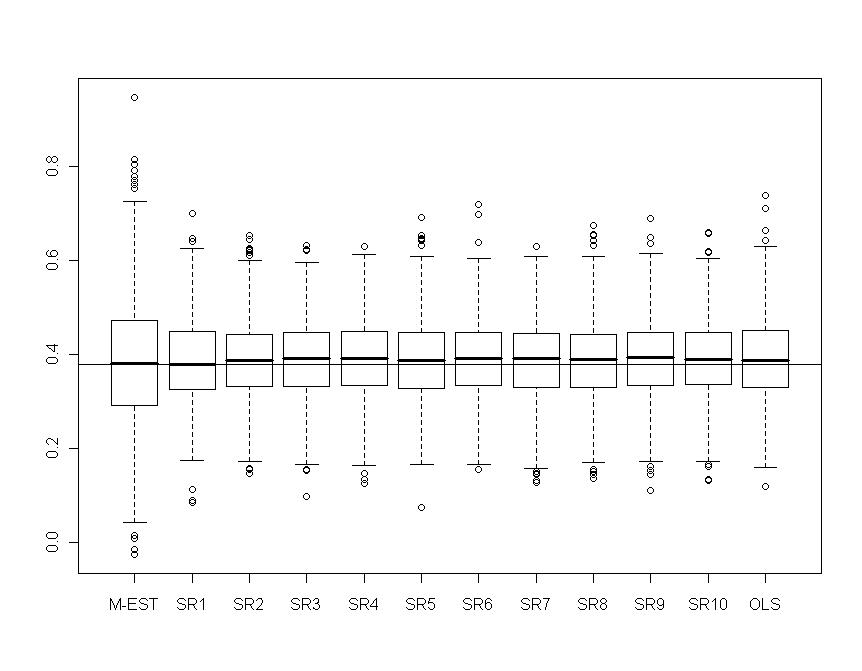
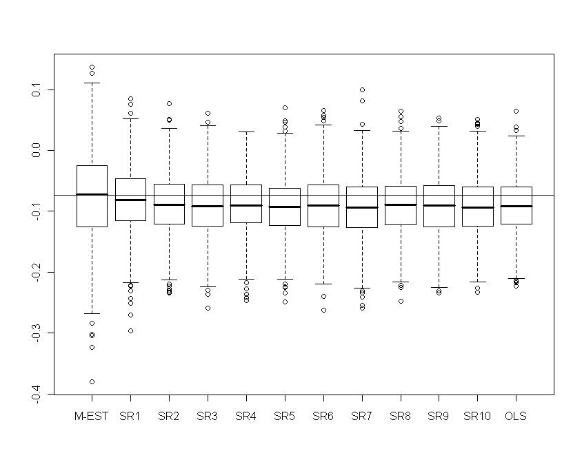
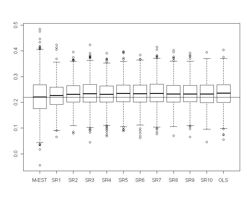
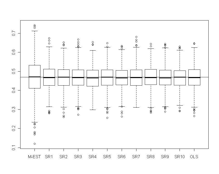
We simulate 1000 training data sets of size each and containing the same kind of contamination. For each sample we estimate by M-estimator, OLS and with . Figures 10-13 show boxplots of these estimates over the 1000 simulated training data. We observe that the shrinkage estimators of and show the biasing effects but those are much less important than in non-constrained regression as presented in section 5. The other effect we can see is that variabilities are large but we observe reduction of variability with some values of the shrinking constant .

Figure 9. Portfolio with normal contamination: relative gains obtained with shrinkage robust estimators compared to M-estimator and OLS on various measures of prediction (RMSE, MAE, STAE)

Figure 10. Portfolio with normal contamination: Boxplots of for several values of shrinkage

Figure 11. Portfolio with normal contamination: Boxplots of for several values of shrinkage

Figure 12. Portfolio with normal contamination: Boxplots of for several values of shrinkage

Figure 13. Portfolio with normal contamination: Boxplots of for several values of shrinkage

Now in Table 2 we report the frequencies of selection of a minimum measure of prediction for a range of values of over the 1000 replicates. The optimal which minimizes the quality of prediction is around 1 for the three measures MAE, RMSE and STAE. At this stage, our simulations showed that with weaker contamination M-estimation is optimal and with less percentage of contamination the optima are very instable.

Table 2. Portfolio with normal contamination: frequencies of selection of a minimum measure of prediction

6.2. Skew-Normal and Skew-t Data

In this example, we suppose that returns are generated from a 4-dimensional skew-normal distribution:

(30)

with parameters:

(31)

We simulate a skew-normal test sample of size and take to be the expended return of the portfolio as in the last subsection. The robust estimate of is:

(32)

The estimated weights are the following:

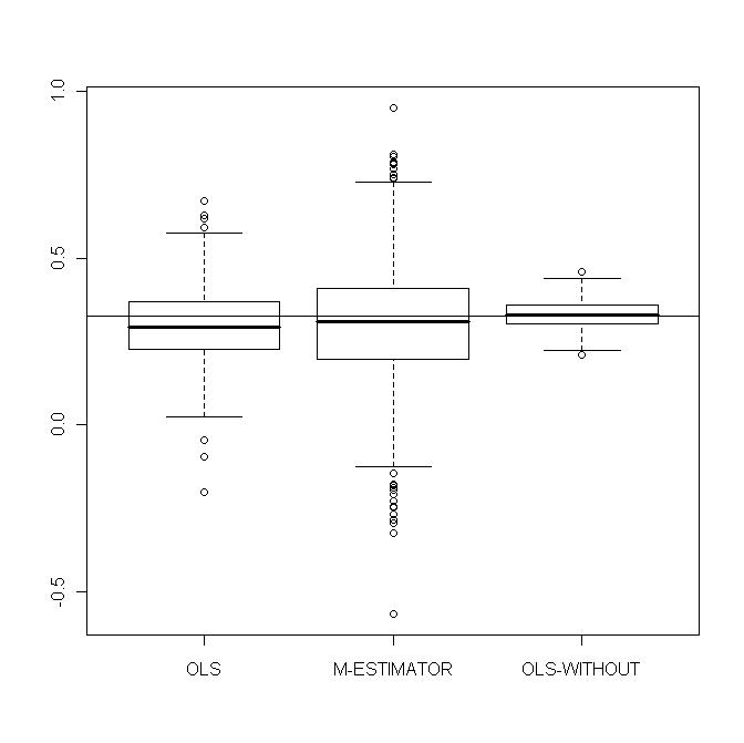
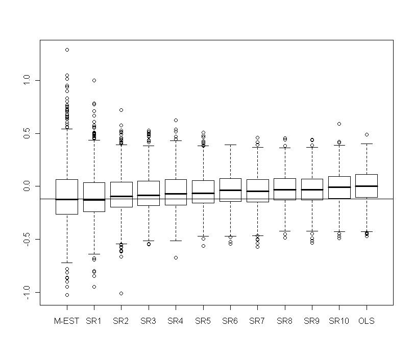
As before we simulate 1000 training data sets of size each and containing the same kind of contamination. For each sample we estimate by M-estimator, OLS and with . Figures 15-18 show boxplots of these estimates over the 1000 simulated training data. We observe that the shrinkage estimators of and show the biasing effect when tends to OLS. Now the IRQ are smaller than in the normal contamination case. The IRQ are in general less than 0.1 excepting the IRQ for which is around 0.2 for the M-estimator. As before we observe the reduction of variability with some values of the shrinking constant .

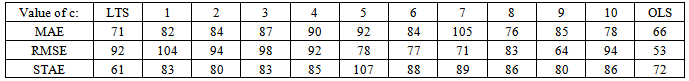
Now in Table 3 we report the frequencies of selection of a minimum measure of prediction for a range of values of over the 1000 replicates. The optimal which minimizes the quality of prediction for MAE and STAE is 1, for RMSE it is around 5. Others simulations showed that these optimum values are more or less instable around 2.

Figure 14. Portfolio with skew-normal returns: relative gains obtained with shrinkage robust estimators compared to M-estimator and OLS on various measures of prediction (RMSE, MAE, STAE)

Figure 15. Portfolio with skew-normal returns: Boxplots of for several values of shrinkage

Figure 16. Portfolio with skew-normal returns: Boxplots of for several values of shrinkage

Figure 17. Portfolio with skew-normal returns: Boxplots of for several values of shrinkage

Figure 18. Portfolio with skew-normal returns: Boxplots of for several values of shrinkage

Table 3. Portfolio skew-normal contamination: frequencies of selection of a minimum measure of prediction

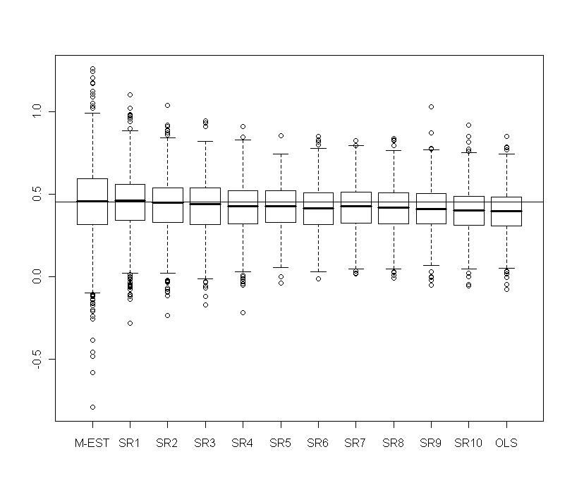
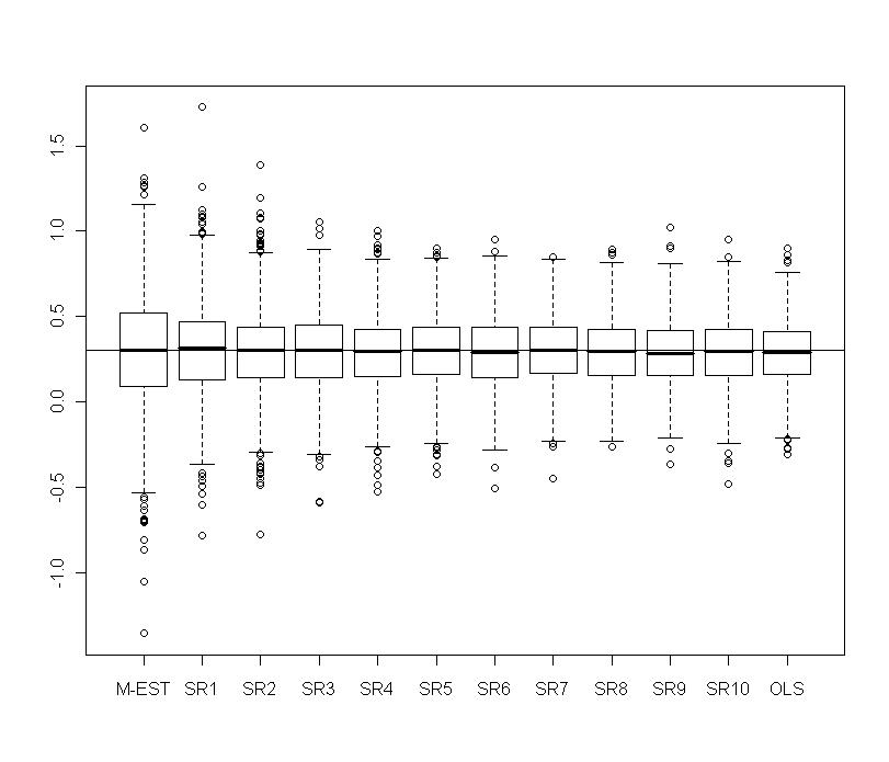
Finally, Table 4 summarizes the computations for the Skew- model, using the same parameters as the skew-normal and using 3 degrees of freedom. Small degree of freedom value allows for more outliers. Following Huisman thesis (1999), 3 to 6 degrees of freedom are usual in finalcial data. The optimum value for is about 5.

Table 4. Portfolio skew-t contamination: frequencies of selection of a minimum measure of prediction

7. Conclusions

In this paper, we have implemented a multivariate version of the shrinkage robust estimators described in Genton and Ronchetti (2008). The aim was to apply the method to the estimation of weights for portfolio optimization. The greatest difficulty was to combine the general method with the constraints which are present in the definition of portfolio optimization. We have seen in Section 6 that the shrinkage constant is more instable than in the non-constrained case (Section 5). The origin of the effect is very probably the high instability of the estimation of portfolio weights even with M-estimators. Anyway, the simulations show a optimal shrinkage constant of about 1 for our skew-normal returns and about 5 for our skew-t returns. Location, scale and shape parameters were the same for both laws. We used a skew-t distribution with 3 degrees of freedom, and consequently large outliers were allowed.

The Monte Carlo simulations give us only empirical heuristics for actual applications of the robust portfolio allocation. In the future this can be followed by a theoretical study to find more general properties relating asymmetry and shrinkage.

ACKNOWLEDGEMENTS

The core of this work was done while the author was a master student in statistics in the University of Geneva in 2008. The author is very grateful to Prof. Marc Genton and Prof. Elvezio Ronchetti for helpful advises and remarks.