1. Introduction & Motivation

The stock market crash of 1929 was so swift and the economic and social consequences of its aftermath so severe that memories from that period of time have, to a significant degree, been passed down to subsequent generations. The episode remains a hallmark of American economic turmoil (Klein, 2001). Historical studies have extensively covered the events before and after the crash and documented the consequences of it (e. g. Helder, 1974). In spite of extensive study, some key issues concerning the Great Crash remain contested. Among them, one is of central importance for our paper: Did a bubble cause the stock market crash of 1929?

The answer leads to related and more general questions at the heart of financial economics, namely: are markets inherently unstable and cause bubbles that may result in economic disasters like the Great Depression when they unwind, or do stocks follow the Efficient Market Hypothesis with stock prices accurately representing all public information on the stocks’ relevant underlying fundamentals?

Historical accounts of the Great Crash of 1929 (Galbraith, 1961; Wigmore, 1985; Rappoport and White, 1993, 1994; Klein, 2003; Ahamed, 2009; Kindleberger and Aliber, 2011, among others) tend to describe the years preceding the Great Crash as a bull market. Stock prices went up because further price increases were anticipated and investors were in search of those perceived capital gains (more or less along the theoretical lines of Allen and Gorton, 1993, and the momentum strategies empirically tested by Chan et al., 1996), thus providing an unambiguously affirmative answer to the question posed above about the existence of a bull market in the years before the 1929 Crash.

The reasons behind the Crash are not so clear-cut in the specialized financial economics literature. Santoni (1987) examined the percent changes in the Dow Jones Industrial Index (DJIA) around the time of the so-called ‘Coolidge bull market’ (1928-1929) and found no evidence of a speculative bubble. Similarly, Diba and Grossman (1987) found that stock prices and dividend payments were non- stationary in their levels but stationary in their first differences during the years of the Great Crash. The finding is an indication of the presence of random walks and thus negates the possibility of a bubble. In spite of a few papers presenting contrarian evidence (De Long and Shleifer, 1991, for instance), the consensus in the financial economic literature during the 1990s showed there was no clear evidence for bubbles at all, not only in the case of the market implosion of 1929, but for any episode (see the discussion in Rappoport and White, 1993, or refer to Fama, 1995a, Donaldson and Kamstra, 1996, among others, for additional examples). Even in the 2000s, a period marking the ascent of behavioral financial economics, no shortage of papers showing general skepticism toward bubbles in general (Meltzer, 2003, for instance), denying the existence of a bubble during the years of the so-called Great Crash (McGrattan and Prescott, 2000, 2001, 2003, and 2004, for example), or reaffirming the general empirical validity of the efficient markets hypothesis/no bubbles view of the world (Rubinstein, 2001, Malkiel, 2003; Yen and Lee, 2008) occurred.

What accounts for these ambiguous results between the two strands of literature? In our view, ambiguity in assessing the Great Crash arises in part from the nature of the time series data, tests, and analyses that economists were able to use in the past. At least four issues stand out. First, the highly aggregated data, generally used, prevented a more careful study of the specific origins of the price shocks at the company level and restricted researchers to the analysis of highly aggregated indexes, such as the Dow Jones Industrial Average (DJIA). The results may have conflated the existence of true price bubbles at lower levels of aggregation. Second, low frequency data (typically annual data) prevented a more careful examination of the short-term price dynamics in place and created a derived third problem, namely the excessively long period of study being used (typically the period between 1920 to 1925., In such a long period, stock prices and dividends stayed quite in line with one another (especially in the years 1920-26), thus biasing the tests toward the rejection of the hypothesis that a bubble existed. Lastly, the inadequacy of the stationarity and unit root tests applied to the price series made the rejection of the null hypothesis of no price stationarity very difficult, given the low power and size distortion issues characteristic of the ADF and PP tests (De Jong et al., 1992, Schwert, 1989).

In this paper, we revisit the case of the Great Crash of 1929 and address the four issues raised above. We first make use of disaggregated data at the company level from the WRDS database, maintained by the Wharton School of Business. We examine the transmission of price shocks from certain key companies that historians have identified as the critical ones leading the financial cycle to the rest of the companies in the DJIA in a way that, to the best of our knowledge, is new in the literature. Second, by being able to use monthly data we can both better study short-run price dynamics and also restrict the period of study to the one that historians have already identified as the critical one (1926-33). Finally, by making use of stationarity tests, such as the KPSS test (Kwiatkowski et al, 1992), and unit root tests, such as the ERS test (Elliott et al., 1996), we can benefit from statistical tools that do not suffer from the same well-known problems (lack of power to reject the null of no stationarity and size distortions) than the ones that have been mostly used before.

Our paper is organized as follows: Section 2 presents our data and methodology to test for the presence or absence of random walks in the stock price data. Section 3 presents the main empirical results of this study and is divided into 5 subsections. Subsection 3.1. presents the results of both the KPSS stationarity tests and ERS unit root tests applied to 24 publicly traded companies in the New York Stock Exchange during the period between December 1925 and December 1933. Subsection 3.2. presents Granger causality tests documenting the origins of the price shocks at the company level. Subsection 3.3. documents how the price shocks spread qualitatively across companies after having started in a handful of highly innovative new companies. Subsection 3.4. documents the quantitative impact of the price shocks, by means of impulse-response analyses. Subsection 3.5. documents the long-term consequences of the crash in the form of highly persistent price undershooting for many of the stocks analyzed. Section 4 discusses the relevance of our results for the financial economics literature (both the specific one studying the Great Crash, and the one studying bubbles in general). Section five closes with suggestions for further research.

2. Data and Methodology to Test for Random Walks in Stock Prices

For our empirical analysis, we used monthly data from the WRDS database maintained by the Wharton School of Business of the University of Pennsylvania. In total we assembled data for 24 companies. We classified our entire dataset in three different subsets for the purpose of analysis. Our first subset consists of all of the companies included in the Dow Jones Industrial Average (DJIA), as of 12/07/1925 for which information was available in the WRDS database. Selecting companies according to such an exogenous criterion minimizes the risk of sample selection and survivorship biases. On the downside, though, it leaves smaller companies out of the subset. Specifically, the DJIA index consisted of 20 companies as of 12/07/1925. Out of these 20 companies the WRSD database did not contain information for 5 of them (American Smelting, American Tobacco, Mack Trucks, Western Union, American Telephone and Telegraph Company). General Motors is also excluded from this subset, since it is included in our third subset, called “Innovative companies” (see below). In sum, the companies included in the Dow Jones as of December 1925 for which information was available for the period December 1925-December 1933 in the WRDS database are the following 14: Allied Chemical, American Can, American Car & Foundry, American Locomotive, American Sugar Refining, General Electric, International Harvester, Kennecott, Paramount, Sears, Texas, US Rubber, U.S. Steel, Woolworth. We will be referring to this group of companies as “Subset 1”.

The second subset of companies consists of companies that belong to “traditional sectors” like steel and railroad industries, and were not part of the DJIA as of December 1925. We chose the companies in this subset based on our readings of historical accounts (Wigmore (1985), Rappoport and White (1993), Ahamed (2009), among others), and searched for the availability of those companies in the WRDS database as our readings and learning about the 1929-33 episode progressed. We mainly use this subset of companies as a robustness check to the results obtained using subset 1. Subset 2 is comprised of 8 companies, namely: Bethlehem Steel, Pennsylvania Railroad, Canadian Pacific Railroad, American Woolen, Reynolds Tobacco, Standard Oil California, Lambert Consumption, and Goodyear. From here and thereafter we will be referring to this group of companies, as “Subset 2.” On the upside, this subset is more homogeneous than the first one in that it only contains companies in well-established sectors as of the beginning of our sample, according to historical evidence. On the downside, there is some risk of sample selection bias and, to a certain degree, survivorship bias, as well. Bethlehem Steel, American Woolen, Lambert Consumption, for instance, no longer exist, which provides some assurance that our subset 2 is not entirely chosen based on exclusive information availability pertaining to companies that only exist today.

The third subset contains 4 companies, in particular RCA, Union Carbide, DuPont, and GM, as of December 1925. The criteria by which they were chosen are that all of them have introduced qualitatively radical innovations, by means of technologies that allowed for the production of new goods that led to the creation of completely new economic sectors. The criteria amount to complying with a technological ‘displacement’ a la Minsky (1982). More details on these innovations are mentioned later on in this study (subsection 2.1.). We will be referring to this group of companies from now on as the “Innovative companies.”

2.1. The Selection of the Four Qualitatively Innovative Companies

Unlike Nicholas (2008), who defines innovation based on the number of patents under each company’s name, we choose the subset of innovative companies using a qualitative criterion, not a quantitative one. We follow Minsky (1982) and Kindleberger and Aliber (2011) and use the concept of ‘technological displacement’ to select our subset of innovative companies. According to Kindleberger-Minsky, a technological displacement is a shock that has the potential to capture investors’ imagination leading them to believe with some degree of empirical plausibility that the radically new technologies, goods, and sectors being introduced give rise to a fundamentally different world, one in which stock valuations have to be totally reassessed, thus opening the possibility for the start of a price bubble.

In what follows we explain the reasons why we chose these four innovative companies.

The Radio Corporation of America (RCA) was formed in 1919 by the incorporation of the assets of Marconi Wireless Telegraph Company of America, the Pan-American Telegraph Company, and assets already controlled by the United States Navy, leading to a new publicly held company formed by General Electric (which owned a controlling interest) on 17 October 1919. The end of the government monopoly of the radio airwaves at the end of World War I in 1918 led to the formation of a private monopoly over the radio airwaves involving the cooperation of the recently formed RCA with General Electric, the United Fruit Company, the Westinghouse Electric Corporation, and American Telephone & Telegraph (AT&T). By 1926 the market for commercial radio expanded, and RCA purchased radio stations and networks from AT&T, and merged them with a chain of stations in New York and Washington, leading to the formation of the National Broadcasting Company (NBC), the first national network of radio stations. Both Westinghouse and GE used RCA as their retail arm for radio sales. RCA also introduced the sound film technology known as photophone, the first commercially viable technology to synchronize sound and picture motion in films (Wigmore, 1985). Lastly, RCA also pioneered the creation of color TV in 1927. The idea of television was not new, and mechanical systems had demonstrated its feasibility by means of crude pictures. But it was engineers David Sarnoff and Vladimir Zworykin’s historic meeting that set the stage for RCA’s success at perfecting electronic television transmission and reception. The importance of this innovation should not be underestimated. Indeed, David Sarnoff himself publicly speculated on the possibility of “every farmhouse equipped not only with a sound-receiving device but with a screen that would mirror the sights of life” (RCA, n.d.), a thought which perfectly illustrates the ability of dramatic qualitative innovations of the type Minsky and Kindleberger had in mind as ways to capture peoples’ imaginations and eventually lead to price bubbles. Indeed, according to Galbraith (1961, p. 51), in 1929 an advertisement in the New York Times called attention to the impending arrival of television and presciently said that the “commercial possibilities of this new art defy imagination.” According to Galbraith, (1961, p. 51), the ad also opined, somewhat less presciently, that “TV sets would be in use in homes that fall.”

The Union Carbide and Carbon Corporation (currently Union Carbide) was formed in 1917 from the merger of the former Union Carbide, founded in 1898, and the National Carbon Company founded in 1886. In the United States, semi-commercial production of ethylene glycol started in 1917. In 1920 Union Carbide set up a chemicals division which started to manufacture ethylene glycol in 1923 for use as automotive antifreeze, the first one ever used in cars. The first large scale commercial glycol plant was built in 1925 by Union Carbide at South Charleston, West Virginia. By 1929, ethylene glycol was being used by almost all dynamite manufacturers, as well. The invention and commercial success of ethylene glycol was highly complementary of the widespread adoption of the motor car as a popular means of transportation, another hallmark of the 1920s. Data for the Ford Motor Co. are not available in the WRDS database, but the data for General Motors are available, and the second half of the 1920s are the years in which both General Motors and the market for motor cars display exponential growth (The History of AmericanTechnology, n.d.)

General Motors was founded on September 16, 1908, in Flint, Michigan, as a holding company for Buick, then controlled by William C. Durant. At the turn of the 20th century there were fewer than 8,000 automobiles in the U.S. and Durant had become a leading manufacturer of horse-drawn vehicles in Flint, MI, before making his entry into the automotive industry (Gustin, 2012). To get a sense of the gigantic increase in the size of the domestic market for motor cars, it is useful to note that by 1923 GM sold 800,000 vehicles according to The History of American Technology, The Automobile Industry, 1920 – 1929. Also, according to the company’s website “as demand for automobiles grew to unexpected heights in the 1920s, General Motors set the pace of production, design, and marketing innovation for others to follow (General Motors, n.d.) For example, in the 1920s, GM introduced Chevrolet, Vauxhall and Opel to their lineup of car models as smaller vehicles, thus diversifying the selection and adding to the reach of GM. According to the company’s website, GM followed a philosophy of “a car for every purse and purpose,” and through a series of landmark innovations, changed the automobile industry itself. In 1927 GM introduced the Cadillac LaSalle, a curvy and sporty-looking model, which made people see cars as much more than just a mode of transport, marking the beginning of true automotive design (General Motors, n.d.)

Another sector that saw great qualitative breakthroughs was the chemical industry, and DuPont was the leading innovator, with breakthroughs that impacted the clothing and food industries in decisive ways (Nicholas, 2008). DuPont was founded in 1802, using capital and machinery imported from France. It started as a company that manufactured gunpowder, but the company eventually shifted its focus toward chemicals, a sector in which it had a series of decisive breakthroughs in the 1920s. DuPont put its emphasis on developing the science of materials, polymers in particular, inventing neoprene, the first synthetic rubber, and the first polyester super-polymer. These innovations radically transformed the clothing industry in the 1920s, giving rise to a new sector, namely the one of high performance clothing. Another important polymer introduced by DuPont in the U.S. in 1923 was cellophane, a material that impacted the retailing of food, by allowing producers and retailers to attractively display their products and also allowing consumers to see what they were buying (Dutton, 1949).

A word of caution is in order at this point in regards to our list of qualitative innovators. Our list is not an exhaustive one. There may be a few other qualitative innovators that we may have been unable to identify, either because the data are not available in the WRDS database, such as is the case for Ford Motors Co., as already mentioned, as well as Columbia Graphophone, and AT&T, or because we have been unable so far to find enough reliable sources of information to justify their inclusion. In particular, Wright Aeronautics, and Montgomery Ward, a chain store, are worth mentioning as candidate companies for future inclusion, as they are mentioned by some historical sources, but significantly more research is needed before they can be included in the analysis.

2.2. Data Sources

All the data used in this paper comes from the Wharton Research Data Services.

2.3. Data Graphs – Price and Dividend Payments

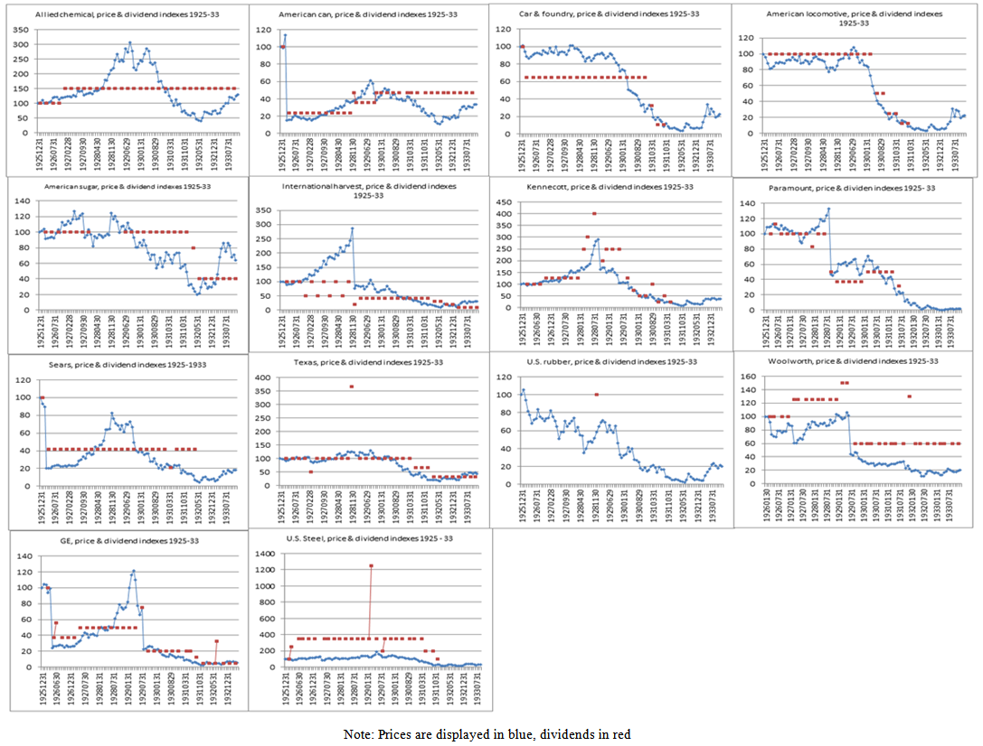
Nine companies from Subset 1 start showing a close association between price and dividends at the beginning of our sample period (1925-1933). However the link for all of them breaks at different points either during 1926 or at some point in 1927. After 1927 those nine companies showed prices that clearly divorced from dividends. These nine companies are: Allied Chemical, American Can, American Locomotive, American Sugar, International Harvester, Kennecott, Paramount, Texas, and GE. Another two companies (Sears, and American Car & Foundry) provided a textbook example of a Shiller (1981)-type violation of weak efficient market hypothesis (EMH), since their prices fluctuated wildly while dividends stayed constant for the entire period. Yet another company that provides a clear violation of the EMH was U.S. Rubber that paid dividends only once but had prices fluctuate significantly for the entire period.

Figure 1. Price & Dividend Indexes, 1925-33 – Subset 1

The general picture from Subset 2, shown in Figure 2, suggests that there is no association between prices and dividends even at the beginning of the sample, except perhaps in the case of Pennsylvania Railroad. One extreme case highlighting the divorce between price and fundamentals is given by American Woolen, a company that paid a dividend only once in the entire period and had prices that varied significantly.

Figure 2. Price & Dividend Indexes, 1925-33 – Subset 2

The patterns of price indexes across companies and between subsets of data can be neatly captured by averaging the price indexes across companies in each subset (all averages are not weighted by volume) and comparing the average of the Innovative Companies versus the average of Subset 1 and the average of subset 2. The results of such procedures can be seen below. Figure 3 displays the average price index for subset 1 companies versus the average price index for the Innovative companies, and Figure 4 does the same for the second subset.

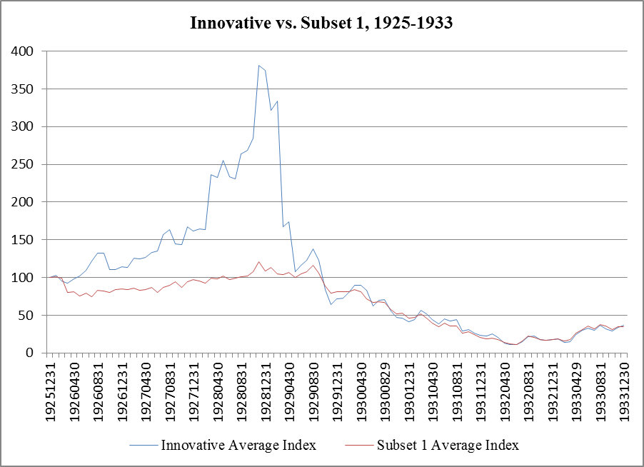Figure 3. Average Price Index of Innovative Companies vs. Average Price Index in Subset 1

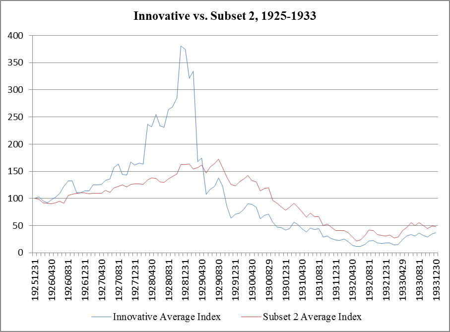Figure 4. Average Price Index of Innovative Companies vs. Average Price Index in Subset 2

2.4. Methodology to Test for Random Walks/weak Market Efficiency

We followed a multi-step procedure to test for the presence or absence of random walks in the stock price data. After plotting all price series and the cash dividend payments series over time for each company to observe the relationship between price and its closest fundamental, we ran simple regressions between price and its first lag. In the vast majority of cases, the estimated coefficients were higher than 0.96 (i.e., very close to unity), suggesting near random walks in all cases, confirming the findings of Fama (1965a, 1965b). Only then we proceeded to test unit for roots by first using KPSS stationarity tests and then re-checking the results by reversing the null hypotheses, a well-known and useful device, by means of ERS unit root tests. The KPSS tests postulate a null hypothesis in each test in which price is stationary (in our case, stationary around a linear trend). The null hypothesis of price stationarity makes a priori sense for two reasons, one economic, one statistical. The economic reason is that all graphs of the time series of price indexes versus cash dividends payments suggested that: (1) there was a deterministic boom-bust pattern in the price data, but not in the dividends data, (2) there was a divergence between price and dividend payments that typically began in 1927; and (3) in almost all cases, the existence of a linear trend in the price series was visually clear and it connected the starting and endpoints of the series. Those facts suggested a lack of a random walk prima facie, and hence, choosing a null hypothesis of price stationarity. From a statistical point of view, it also makes sense to choose a unit root test with a null hypothesis of price stationarity in this case, given that the estimated coefficients were extremely close to unity, leaving the ADF test, the Phillips-Perron test, and all tests in which a unit root is the null hypothesis and the data are not detrended before testing, with a very difficult discriminating task and low power to achieve it (De Jong et al., 1992).

The KPSS tests failed to reject the null hypothesis of price stationarity in all cases but two with an associated risk of accepting a false null hypothesis of 1%. In those two cases, we proceeded to re-ran the original regression in a slightly expanded form, so that the expanded model was of the ARMA (2, 2) form, and we found that the AR(2), MA(1), and MA(2) components helped explain the price of the stocks involved in a significant way, denying the existence of a random walk.

The last step involved re-checking the prior results by means of reversing the null hypothesis and making use of ERS tests. The ERS test is more powerful in unit root tests that cannot distinguish non-stationary processes from highly persistent stationary ones (Elliott, et al., 1996). Results from the ERS tests were even clearer than results from the KPSS tests, and the null hypotheses of unit roots in the price levels were decisively rejected in all cases by margins that left very little room for doubt.

2.5. Methodology to Study Pairwise Granger Causality

To test for the type of causality between the price indexes of traditional and innovative companies, we ran multiple sets of pairwise Granger causality tests.

Since the stock price variables were stationary in their levels (i.e., they did not display unit roots in their levels), Granger causality analyses did not need to be performed within Vector Error Correction Models, and cointegration tests were not called for.

Since RCA is generally regarded by historical accounts as a symbol of the bull market preceding the crash, we choose RCA as the representative innovative company to use in pairwise comparisons with traditional companies. The pairwise causality tests between the other three innovative companies and the traditional companies were qualitatively similar to the ones involving RCA, but to save on space we do not present them here (instead, we make them available upon request from the authors). Instead what we do present below is the effect of the four innovative companies’ (unweighted) average price index on the DJIA index (please see Figure 3 and Table 3 in section 3. 2. below).

Our methodological steps proceeded as follows. First, we applied the pairwise Granger causality tests to identify the exogenous variable in the pairs (RCA, traditional companies in subset 1 and subset 2). The tests were performed by adding cross lags to the pair of auto-regressive equations. Then, checks for the jointly added explanatory power of the cross lag terms in the expanded auto-regressive models were performed by means of the F-test. Then we ran unrestricted VAR models with the optimal number of lags chosen using the Schwartz Information Criterion (SIC), and next we re-ran Granger causality tests by means of the exclusion of variables’ tests based on the Chi-Squared distribution.

Following, we checked whether the inverted roots of the characteristic polynomials were within the unit circle so as to guarantee valid impulse-response functions. Last, accumulated impulse-responses were calculated over different time horizons, namely 12 months (to capture short-term responses), and 48 months (to capture medium-term responses). Variance decompositions were also obtained to check that the qualitative results also had meaningful quantitative value (they are not reported here to save on space, but are available upon request from the authors).

3. Empirical Results

The presentation of the main empirical results is organized around four critical research questions: 1) Was there a bubble or not? 2) If there was a bubble, how did it start? 3) How did the bubble evolve over time? (In other words, how was the bubble transmitted across companies?) 4) What were the consequences of the crash?

3.1. Was There a Bubble?

The short answer is a definitive yes. Our regression analyses show clear evidence that stock prices behaved as near random walks (“approximate random walks” in the choice of words of Fama, 1965) in the period December 1925-December 1933. However, ERS tests rejected the presence of unit roots in the price series decisively. Furthermore, KPSS tests showed overwhelming evidence against exact random walks. In cases in which the peak of the series happens to lie in the middle of the sample, such as in most cases in Table 1 and 2 below, the KPSS tests display severe size distortion and are biased toward rejecting the null of stationarity (Badillo et al., 2002). Nevertheless, as Table 1 below shows, the null hypothesis is still accepted in the majority of cases for companies in subset 1.

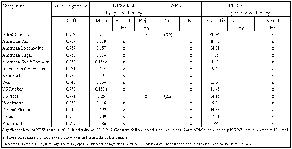Table 1. Unit root for Subset 1, 1925/12-1933/12

Table 2 below summarizes similar evidence for subset 2.

As can be seen in Table 2 below, the bias of the KPSS test to reject the null of stationarity in the presence of a price peak in the middle of the sample is more visible for companies in subset two, as half of them now display rejection of the null hypothesis.

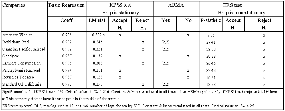Table 2. Unit root tests for Subset 2, 1925/12-1933/12

3.2. How Did the Bubble Start?

The short answer is that it all started with self-induced increases in the stock prices of a few companies pioneering the use of new technologies. These companies’ stock prices displayed temporarily self-sustaining price increases, led the way, and peaked first. Figure 3, on page 12 above, displays the (unweighted) average price index for the four innovative companies in new sectors (RCA, Union Carbide, GM, and DuPont) versus the average Dow Jones Index.

As Figure 3 clearly illustrates, the 4 companies’ price indexes started to increase first and reached their peaks before the Dow Jones Index. Table 3 shows Granger causality tests confirming the temporal precedence of the price increases of these 4 innovative companies over the Dow Jones index. Causality is unidirectional in all four cases. All four companies in new sectors, namely RCA, Union Carbide, GM, and DuPont Granger-cause the Dow Jones, but the Dow Jones does not Granger-cause any of these four companies.

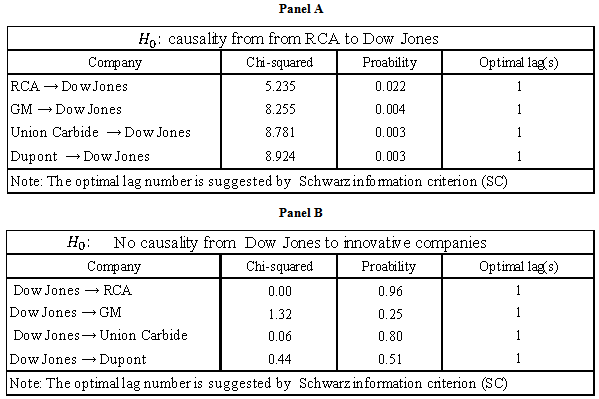Table 3. Granger Causality test between Innovative companies and Dow Jones

3.3. How Did the Bubble Spread?

What emerged as a relatively clear pattern were the following connections: (1) <Innovative companies → Subset 1 companies>, and: (2) <Innovative companies → Subset 2 companies>

Innovative Companies to Traditional Companies Granger causality evidence

In our first subset, based on companies in the Dow Jones, there is evidence that the boom started in the companies operating in new sectors and was transmitted later to many individual companies operating in traditional sectors. As a representative example, we show evidence that RCA Granger-caused seven companies in the Dow Jones (GE, US Steel, US Rubber, Sears, Allied Chemical, American Can, and American Locomotive), and caused and was caused in another three cases of companies included in the Dow Jones (Woolworth, Kennecott, and International Harvester). Only in two cases we observed reversed causation from traditional companies in the Dow Jones (Texas and Paramount) to RCA, and only in two cases no pattern of causation could be identified (those were the cases of American Car & Foundry and American Sugar). Table 4 (panels A & B) summarizes this evidence.

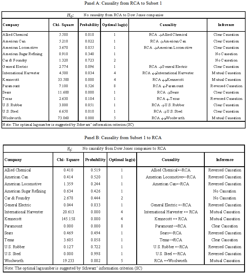Table 4. Granger causality between RCA and Subset 1

In our second subset, RCA Granger-caused all but one of the traditional companies outside the Dow Jones, namely Reynolds Tobacco. In the case of Reynolds Tobacco, RCA caused and was caused by it. In almost all cases, the optimal lag structure involved just one lag, contrary to what was the case in the Dow Jones subset in which the lag structure was frequently richer. Table 5 summarizes this evidence.

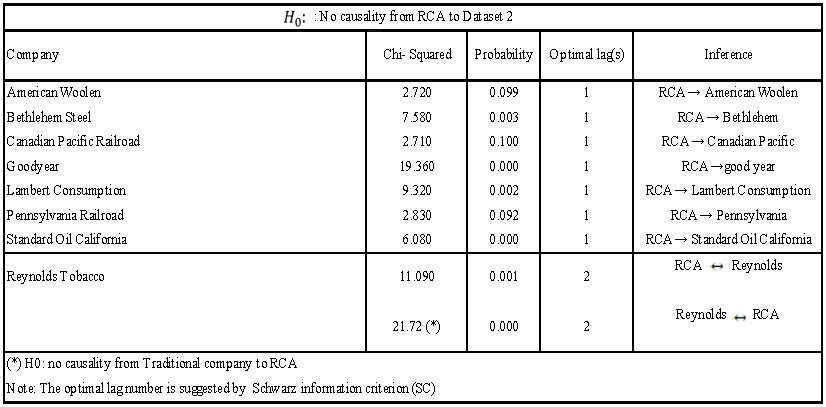Table 5. Granger causality between RCA and Subset 2

3.4. Impulse Responses

In order to isolate the effects of orthogonalized shocks from RCA to traditional companies, we entered RCA first in the Cholesky factorization, according to the Granger causality results reported in the previous section. Accumulated impulse-responses are displayed in two different panels. To capture the short-run responses, a 12-month panel is displayed in each table. To capture the medium-term responses, we choose a panel with a window of 48 months. Finally, in order to save space, we only report ‘cross-companies’ accumulated responses. In other words, responses of companies to their own price shocks are not reported.

Accumulated impulse-responses from Panel A, Figure 5, show that a one standard deviation increase to the price of RCA leads to twelve of the fourteen companies in Subset 1 to display price increases during the first twelve months after the shock to the price of RCA (the only two exceptions are Paramount and International Harvester). The largest quantitative response was the one by Allied Chemical with a gain of 120 points in the first 12 months after the shock to the price of RCA. On average, the majority of companies displayed gains in the range of twenty to sixty points. Accumulated impulse-responses from Panel B, Figure 5, show that after 48 months the qualitative patterns remain quite similar to those in Panel A. Interestingly Allied Chemical accumulated gains for roughly 200 points.

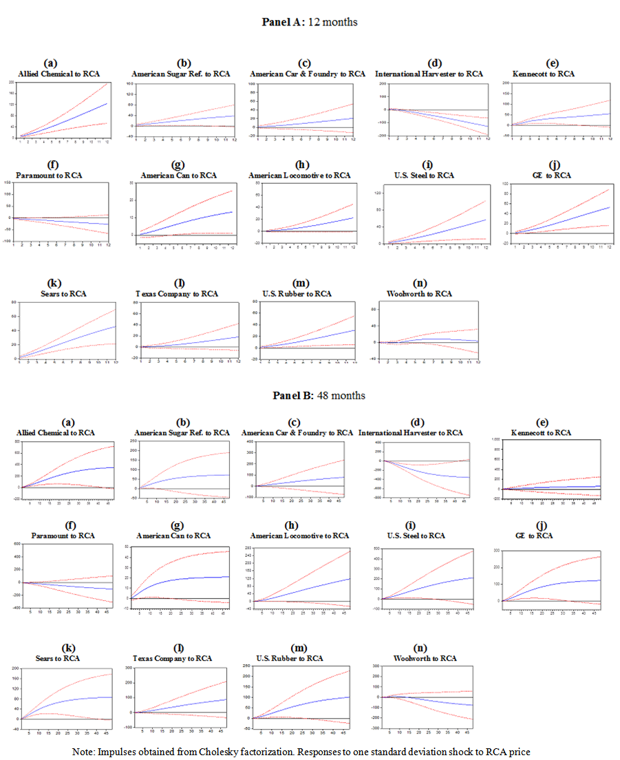Figure 5. Accumulated Responses of Dow Jones’ companies to RCA Impulses

Accumulated impulse-responses from Panel A, Figure 6, show that a one standard deviation increase to the price of RCA leads to 7 of the 8 companies in Subset 2 displaying price increases during the first twelve month after the shock to the price of RCA (the only one exception is Reynolds Tobacco). The companies outside the Dow Jones seem to have a larger quantitative response to the shocks from RCA price. For example, three companies (Goodyear, Lambert Consumption, and Union Carbide) showed price gains in the range of 150 points 12 months after the shock to the price of RCA.

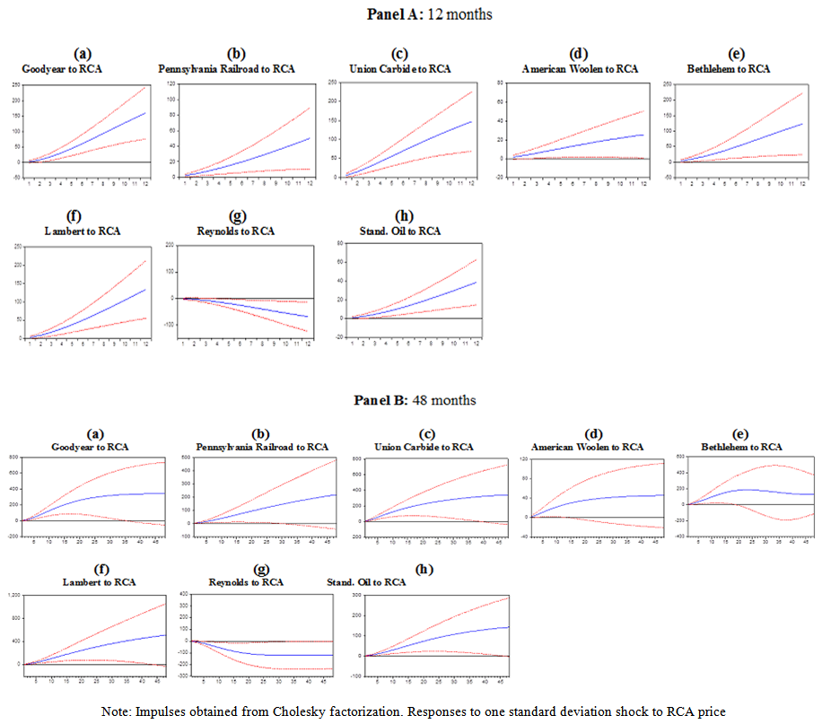Figure 6. Impulse Responses of subset 2 companies to RCA Price Index

In a period of 48 months after the shock to the price of RCA, shown in Panel B, Figure 6, most of the companies display accumulated gains in excess of 200 points, with the exception of American Woolen, Reynolds Tobacco, Standard Oil California, and Bethlehem Steel.

Turning to Figure 7 accumulated responses show that the average price of the Dow Jones’ companies increased about 50 points during the first 12 months after the shock to RCA’s price, and roughly a 150 point gain 48 months after the shock to the price of RCA. Since four companies that belonged in the Dow Jones as of December 1925 are missing in Subset 1, we checked that their absence did not significantly change our results by calculating the response of the entire Dow Jones Industrial Average Index to a one standard deviation change to the price of RCA. We do not include those graphs to save on space but results were as follows: The accumulated response of the DJIA after 12 months showed a 90 point increase, and a 150 point gain after 48 months. There was literally no feedback response by RCA from the shock to the Dow Jones Industrial Average, either after 12 months or 48 months.

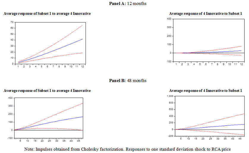Figure 7. Accumulated Impulse Responses: Average Subset 1 vs. Average of 4 Innovators

Similarly, in the case of Subset 2 accumulated responses displayed an increase of 60 points and 200 points after 12 and 48 months, respectively. We observe no feedback response; in other words, innovative companies were not affected by the increase of the price indexes from companies outside the Dow Jones.

3.5. What were the Consequences of the Crash?

The short answer is that the crash was followed by a severe and protracted price undershooting that lasted at least until December 1941, the beginning of the U.S. involvement in World War II, as shown by Figures 9 & 10 below for Subsets 1 and 2, respectively.

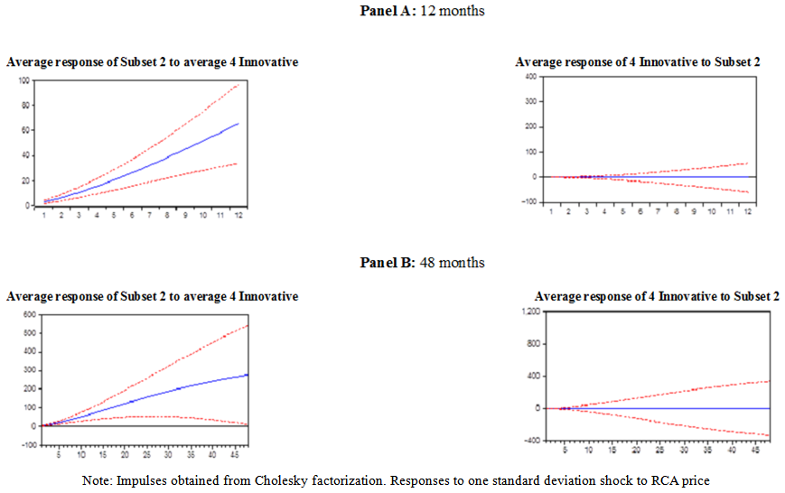Figure 8. Accumulated Impulse Responses: Average Subset 2 vs. Average of 4 Innovators

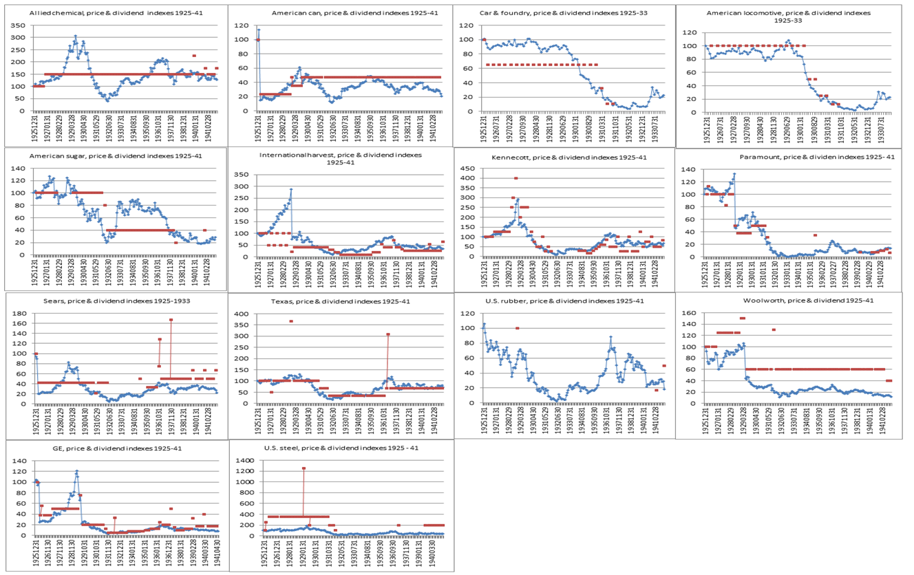Figure 9. Price undershooting until 1941, Subset 1

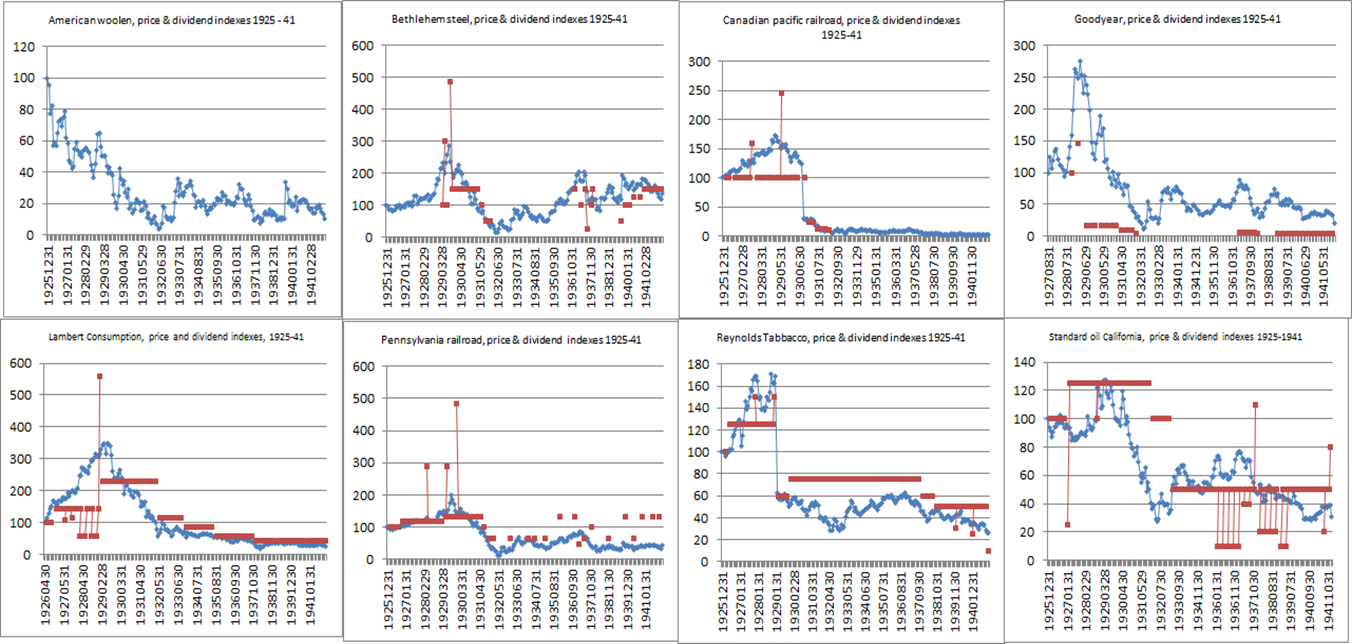Figure 10. Price undershooting until 1941, Subset 2

Figure 9 shows two important pieces of evidence. First, prices stayed depressed after the crash of 1929 until the end of 1941 for 10 out of 14 companies in Subset 1. Second, prices reconciled with dividends for only 5 out of 14 companies after the crash (Allied Chemical, International Harvester, Kennecott, Texas, and GE), and furthermore in three of those 5 cases, namely Allied Chemical, International Harvester, and Kennecott, prices led dividends on the way down, instead of the other way round, as standard theory suggests.

Turning to companies in Subset 2, Figure 10 shows two important pieces of evidence. First, prices stayed depressed until the end of 1941 for 7 out of 8 companies, the exception being Bethlehem Steel. Second, only in the case of two companies (Lambert Consumption and Canadian Pacific Railroad) did prices reconcile with dividends. However, in those two cases, prices seemed to lead dividends, and not the reversed.

4. Discussion and Relevance for Financial Economics Research and Policy

4.1. Unit Root Tests in the Presence of Break Points

We are aware that unit root tests conducted in the presence of break points may produce misleading results. We checked for the presence of break points in two different ways. First, we use a battery of Chow break point tests for different dates (not shown here) and found that in all cases there was a break point coinciding with the peak of the stock price series. Break Point regressions (not shown here) confirmed the results from the Chow tests and partitioned the sample of 98 monthly observations (December 1925-December 1933) into two subsamples of similar size. Results of unit root tests using monthly data for each of the sub-samples around the typical breakpoint showed very similar qualitative outcomes to the ones displayed in Table 1 and Table 2, so long as deterministic trends were allowed in the tests. However, given that each sub-sample is quite short, the reliability of those tests is not the best. To test for unit roots in the best possible way and obtain highly reliable results, the use of daily data will likely be necessary, and that is one of the extensions proposed in the last section of this paper.

4.2. Relevance of Our Research for Minsky’s “displacement” Hypothesis

The evidence presented in Table 4 (panels A, B) and Table 5 seems broadly in line with the existence of a technologically-driven displacement a la Minsky (1982). Nicholas (2008) used the number of patents under each company’s name as his main indicator of innovation and found that it did not correlate well with the price increases observed in the run-up to the Great Crash. We instead tried to use qualitative criteria, an admittedly more risky and elusive exercise, as a first attempt to try to operationalize the Kindleberger-Minsky hypothesis of technological displacement, an issue on which we have been unable to identify much prior research.

4.3. Relevance of Our Study for the Conduct of Lab Experiments on Bubbles

The kind of bubbles that have been studied in the laboratory have all followed in the footsteps of Smith et al. 1988 (Porter and Smith, 1995; Ackert et al. 2001; Haruvy and Noussair, 2006, among others) and are characterized by a period in which prices significantly deviate from fundamentals followed by an eventual convergence between the two. The faithful adherence of subsequent researchers to the original experimental design by Smith et al. (1888) implies that the types of experimental bubbles studied so far cannot have significant and protracted price undershooting after the crash. Why is the issue of price undershooting important? Because there are large economic costs associated with significant and protracted price undershooting. If, as the evidence contained in our time series suggests, prices were roughly aligned with fundamentals by 1926, the fact that they do not return to fundamentals for most of the companies in our dataset for a long time hints that bubbles produce significant economic waste. If the evidence discussed in this study were to be confirmed by other studies, then models of bubbles and experimental bubbles themselves will have to be modified to account for this important feature of real world bubbles.

4.4. Relevance for Financial Economic Theory (EMH)

In this section we extend the sample period of our study until the last data point available in the WRDS database to test for the validity of the random walk hypothesis in a sample that is not dominated by boom-bust dynamics.

Table 6 below presents the results of the KPSS stationarity tests and the ERS unit root tests for the companies in our first Subset. The picture is quite clear: the random walk hypothesis is rejected in a majority of cases. This finding stands in full support of well-established economic literature (Le Roy, 1973; Lucas, 1978). In standard economic theory, such as the C-CAPM model, the EMH hypothesis is just a special restrictive case in which utility is linear and the representative agent is risk-neutral. In the words of Stephen Le Roy (1973, pp. 444-445), “Except under very special circumstances (particularly risk aversion), the martingale property will be violated…and under general conditions there is no rigorous theoretical justification for it available.” Also, reflecting on the Euler equation for consumption from the C-CAPM model, Lucas (1978, p. 1443) concludes that “evidently asset prices themselves do not possess the martingale property…it is clear that the presence of a diminishing marginal rate of substitution of present for future consumption is inconsistent with this property.”

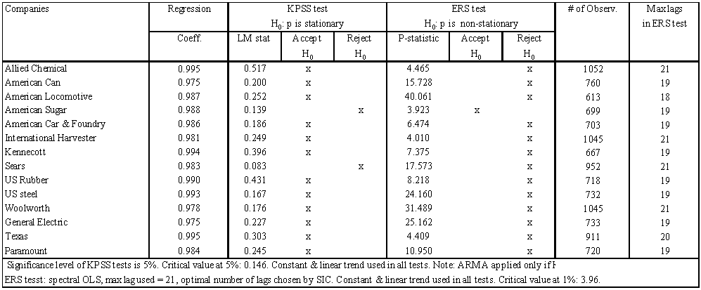Table 6. Unit Root tests-full sample-Subset 1

The picture that emerges from Table 7 below, in which we present the tests of the random walk hypothesis for our second subset, is much more varied than the one for Subset number one. In this case, the random walk hypothesis is rejected almost half the times and accepted for the other half of the companies in the subset, suggesting that the random walk hypothesis retains significant explanatory power under general conditions, if not under the specific ones of the 1926-33 subsample. In a sense, the EMH may be a special case, as noted by Le Roy (1973) and Lucas (1978), but it seems to be an important special case, as also noted by Le Roy (1973) and Lucas (1978).

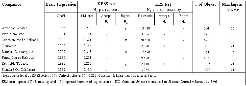Table 7. Unit Root tests-full sample-Subset 2

These findings overlap in part with the ones reported in Vuolteenaho (2002), among the few papers to investigate the issue of bubbles in individual stocks, albeit in an indirect way. Using annual data from the CRSP-Compustat intersection for the period 1954-1996 Vuolteeenaho (2002) uses a panel VAR model to decompose individual stock returns into two components, cash flow news and expected return news and finds that for the typical individual stock the variance of cash flow news is twice the size of the variance of expected return news, suggesting that underlying fundamentals are the largest contributor to the price movements of individual stocks, not the “bubbly” component. Our evidence seems to suggest that this may not be so for a different period of analysis and invites further research on this issue.

5. Concluding Remarks and Open Lines for Further Research

Most of the empirical studies examining whether the crash of 1929 was the consequence of a stock market bubble in the years preceding the crash have assessed the issue using time series data, but have done so with low frequency data and weak unit root tests. Although there has been significant progress in the theoretical time series literature since the mid 1990’s, we have been unable to find papers that apply these innovations to reassess the boom and crash episode centered around the year 1929. Throughout the present study we tried to fill this gap using more disaggregated company-level price data, appropriate unit root tests, and higher frequency time series for stock prices. Our results indicate that a bubble occurred during the years 1927-1929. The cause of the bubble was probably “contagion” from the Innovative Companies towards the more traditional ones.

A central implication of our findings is that investors seemed to be able to anticipate higher future prices during the speculative bubble, which initially encouraged the dynamics of stock prices to deviate from its fundamentals prior to the time of the crash. In particular, our findings regarding the transmission of price shocks from the four innovative companies towards the more traditional ones suggest that these bubbles may have originated in investors’ imagination upon the arrival of new technologies invented by RCA, GM, Union Carbide, and DuPont. This financial contagion spread out rapidly, severely destroyed financial as well as economic values, and lasted at least until the beginning of the U.S. involvement in World War II.

In what follows we suggest a number of interesting extensions to our study. First, we plan to add more companies to the analysis in part to check for the existence of a larger number of highly innovative companies, but also to exploit the cross-sectional dynamics of the data in more depth. Forming a panel dataset would allow for Panel VAR analyses that may uncover the dynamics across companies and sectors in more illuminating ways than pairwise comparisons of time series. Second, we plan to use daily data both to study the very short-run stock price dynamics during the run up and after the crash (admittedly at the cost of adding more short-term noise). We also intend to perform unit root tests in the presence of break points with large sub-samples, a robustness check that requires the use of very high frequency data to increase the number of data points in each of the subsamples around the breakpoint. Additionally, using the methodology advanced by Escobari et al (2013) we would be able to endogenously identify not only the breakpoint at which the bubble bursts, but also the breakpoint at which the bubble starts. Third, we plan to use regime switching regressions to estimate the transition probabilities between boom and crash for each company and for different sectors, and also to estimate the average duration of each regime (that is, boom and bust). Lastly, we plan to add new episodes of booms and crashes with a dual purpose. First, the inclusion of more episodes is useful to continue to test for the existence of bubbles (or lack thereof). Secondly, the inclusion of more cases allows us to keep testing for the Kindleberger-Minsky hypothesis of technological displacement as the potential origin of bubbles. In this regard, we plan to examine the following episodes: the Japanese bull market of the mid to late 1980s, the Asian financial crisis of 1997-98, the Nasdaq tech boom and bust of the mid to late 1990s, and, finally, the crash episode centered around the year 2008 for both the U.S. and Europe.

Note

1. Our data can be found here: http://wrds-web.wharton.upenn.edu/wrds/