1. Introduction

In this paper, we consider a single-server retrial queue with server vacations. We have assumed that the inter-retrial times are generally distributed with a constant retrial policy. After the completion of each service the server goes on a vacation of random length. After the completion of each vacation, the server waits for the next customer. This could be either a primary arrival or the server could try to contact the first customer in the orbit. This is in contrast to the multiple vacation schemes, where the server could take a vacation every time he finds no customers in the system.

An example of such a retrial queuing system is as follows; a service provider (plumber, painter, electrician etc.,) is provided with some mechanism to record the details of the customers requesting service, when he is away attending to some job. After the completion of each service, the provider may take a break before going back to attend to the next customer. Customer requests which arrive during his absence do not wait in a queue but after recording their requirements go away to come back after some time to repeat the request for service.

Motivated by this example, we have therefore considered a retrial queue with a limited single vacation scheme. This scheme is different from the one based on the Bernoulli schedule vacations and applied in the literature by authors like Wang and Li[15], Ebenesar Anna Bagyam and Udaya Chandrika[10].

The rest of the paper is organized as follows: In section-2, we present a brief review of related works in the queueing theory literature. In Sec-3; we present the mathematical model of the system. In Sec-4, we present a steady state analysis of the system and we derive the joint probability generating functions (P.G.F’s) of the server state and orbit size and server state and system size. In Sec-5, we derive the necessary and sufficient condition for the existence of the steady state. In sec-6, we consider some useful performance measures of the system. In Sec-7, numerical results are used to compare numerically the system performance measures with respect to changes of parameters.

2. Literature Review

Retrial queueing systems form an active research area due to their wide applicability in telephone switching system, telecommunication networks and computer networks. Retrial queueing systems are those systems in which arriving customers, who find the server busy, join the retrial queue (orbit) to try again for their requests after sometime.

Retrial queues are useful in modeling many problems in telephone switching systems, computer and communication systems. A review of the literature on retrial queues and their applications can be found in Falin[11] and Yang and Templeton[23], and Artalejo[6]. Two monographs entirely derived to the topic exist and are written by Falin and Templeton[12] and Artalejo and Gomez-Correl[5].

In retrial queueing literature, retrial customers are usually assumed to behave independently and return without regard to other retrial customers. However, Farahmand[13] proposed a special type of retrial system with FCFS retrial queue, that is, if a customer finds the server busy, he may join the tail of a retrial queue in accordance with a first-come-first-served (FCFS) discipline and the customer at the head of the retrial queue would then try again to enter the system, competing with new arrivals. Gomez-Corral[14] considered an M/G/1 retrial queue with a FCFS retrial queue and general retrial times. Single-server queues with vacations have been studied extensively in the past. Comprehensive surveys can be found in Doshi[9] and Takagi[22] and recent developments in vacation queueing Models was introduced by Ke et.al[16], Krishnakumar and Arivudainambi[17]. In our model the server takes a break every time he completes the service. Most of the analyses for retrial queues with vacations concern the exhaustive service schedule (Artalejo[1] and Artalejo and Rodrigo[4]) and the gated service policy (Langaris[20]).Recently, several authors considered retrial queues with Bernoulli schedule, as can be seen in Atencia and Moreno[7], Kumar et al.[18] and Zhou[24]. In this paper we have considered a limited vacation policy. Kasturi Ramanath and K.Kalidass[19] have considered a two phase service M/G/1 vacation queue with general retrial times and non-persistent customers.

In the context of the service provider the limited vacation scheme wherein, the server takes the vacation after each service completion is appropriate. Also, the server cannot take a vacation each time he finds the system empty. The FCFS orbit also makes sense since the server has a record of all the requests that have arrived during his absence. With these ideas we have included a FCFS orbit, a limited single vacation scheme into our model.

3. The Mathematical Model

In this section, we consider a Single-server retrial queuing system with a non-exponential retrial time distribution and with server vacations. Arriving customers to the system are in accordance with a Poisson process with a rate . The service time is generally distributed with a distribution function B(x), Laplace Stieljes transform (LST) and the hazard rate function .

A customer upon arrival, who finds the server free, immediately proceeds for service. Otherwise, the customer leaves the system and joins an orbit from where he/she makes repeated attempts to gain service. The time intervals between two successive retrials are assumed to be generally distributed with a distribution function R(x), hazard rate function and LST R*(s).

We assume that only the customer at the head of the orbit is allowed to make repeated attempts.

We also assume that the elapsed retrial time is measured from the moment the server becomes available for service.

After completion of a service, the server is allowed to take a vacation. The duration of the server vacation is assumed to be generally distributed with a distribution function V(x), a LST V*(s) and a hazard rate function .

We assume that the inter-arrival times, service times, inter-retrial times and the duration of the server vacation are all independent of each other.

Let N (t) denote the number of customers in the orbit at any instant of time t.

Let C (t) denote the state of the server at time t:

In order to make the stochastic process involve into a continuous time Markov process, we employ the supplementary variable technique. This was first introduced by Cox[7]. See Medhi[21] for a detailed explanation of the technique.

We define the supplementary variable X (t) as follows:

We define the following probability functions:

Then is a continuous time Markov process.

4. Steady State Analysis

Now, analysis of our queueing model can be performed with the help of the following Kolmogorov forward equations:

(1)

(2)

(3)

(4)

The boundary conditions are as follows, for n,

(5)

(6)

For

(7)

(8)

Assuming that the system reaches the steady state, the equations (1) to (8) become

(9)

(10)

(11)

(12)

The boundary conditions are as follows for ,

(13)

(14)

For

(15)

(16)

The solution of equation (10) is given by

We define the following partial probability generating functions, for ,

(17)

(18)

(19)

Let

(20)

Theorem: 4.1

In the steady state, the probability generating function of the orbit size is given by

(21)

where and the probability generating function of the system size is given by

(22)

Proof:

Multiplying equation (11) by z and summing over n from 0 to , the solution of the resulting equation is

(23)

Similarly equation (12) gives,

(24)

Similarly equations (13), (14), (15) and (16), we get,

(25)

(26)

(27)

After some algebraic calculations, we get the following values,

(28)

(29)

(30)

Now, from (20),we get,

(31)

(32)

(33)

Hence,

(34)

(35)

(36)

The PGF P (z) of the orbit size is given by

(37)

To obtain the value of , we use the normalizing condition P (1) =1.

Applying L’Hospital’s rule in an appropriate place we get

(38)

Hence

(39)

Let K (z) be the PGF of the system size

(40)

5. The Embedded Markov Chain

In this section, we derive the necessary and sufficient condition for stability of our system. We consider the embedded Markov chain of the process.

Let be the number of customers in the orbit immediately after the service completion epoch . Then if the customer is a retrial customer, otherwise , whereis the number of arrivals into the orbit during the vacation time of the server and is the number of customers arriving into the orbit during the service time of the customer.

By our assumption, the arrival process is independent of the service mechanism and of the vacations of the server and of the retrial processes initiated by the customers in the orbit. Therefore is a Markov chain. The system is ergodic if and only if the embedded Markov chain is ergodic. To prove that the embedded Markov chain is ergodic,we employ Foster’s criterion whose statement is given below:

Foster’s criterion: For an irreducible and aperiodic Markov chain with state space S, a sufficient condition for ergodocity is the existence of a non-negative function f(s), and such that the mean drift is finite for all and for all except perhaps a finite number.

Theorem 5.1: The necessary and sufficient condition for the system considered in the previous section to be ergodic is given by .

6. Performance Measures

In this section, we examine some useful performance measures of the system.

(a) The expected number of customers in the system is given by

(b) The expected number of customers in the orbit

The steady state distribution of the server state is given by

=Prob {server is idle} =.

=Prob {server is busy} ==.

=Prob {server is on vacation} = .

7. Numerical Illustrations

In order to verify the efficiency of our analytical results, we perform numerical experiments by using MAPLE. In this section, we present some numerical examples to illustrate the effect of varying the parameters on the following performance characteristics of our system. We consider the performance measures: the probabilities q₀, q_1, q₂ are the probabilities of the server being idle, the busy and on vacation respectively. We also consider the expected number of customers in the orbit, expected number of customers in the system and . Moreover, for the purpose of numerical illustrations, we assume that the arrival process is Poisson with parametervarying from 0.1 to 0.7, the service time distribution function is exponential with mean = 0.3, the retrial times follow an exponential distribution with LST with parameter =0.8.The vacation time is also exponentially distributed with mean = 0.25.

In all the cases, the parametric values are chosen to satisfy the stability condition.

Example 1:

In this example, we study the effect of varying the arrival rate λ.

From table 1, we observe that if the value of increases, the probabilities of idle time- and decrease. The probabilities of busy time, expected no. of customers in the system and the expected no. of customers in the orbit also increase.

The graph for the data given in table 1 is given below;

Table 1. Effect of varying λ on various performance measures

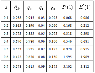
Figure 1. Effect of varying λ on various performance measures

Fig (1.1) shows how (i.e.) the probability of no customers in the system and the server is idle decreases with increasing values of . Similarly, Fig(1.2) shows how the proportion of idle time of the server decreases with increasing values of . Fig (1.3), Fig (1.4), Fig (1.5) and Fig (1.6) show how the server’s busy period and vacation period probabilities, the expected number of customers in the system and the expected number of customers in the orbit increase with increasing values of λ.

Next, we assume that the arrival process is exponentially distributed with parameter =0.1, the service time distribution function is exponential with mean varying from 0.3 to 0.9, the retrial times follow an exponential distribution with LST with parameter =0.8.The vacation time is also exponentially distributed with a mean = 0.25.

Example 2:

In this example, we study the effect of varying the service rate .

From the Table-2, we observe that if the value of increases, the probabilities of idle time- and are decrease and the probabilities of busy time, expected no. of customers in the system and the ,expected no. of customers in the orbit increase.

Fig(2.1) shows how (i.e.) the probability of no customers in the system and the server is idle decreases with increasing values of . Similarly, Fig(2.2) shows how the idle time probability of the server decreases with increasing values of . Fig (2.3), Fig (2.4), Fig (2.5) shows how the server’s busy period probability, vacation time probability and the expected number of customers in the orbit increases with increasing values of . Fig (2.6) shows how the expected numbers of customers in the system increases.

Table 2. Effect of varying       on various performance measures

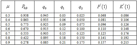
Figure 2. Effect of varying on various performance measures

8. Conclusions

In this paper, we have studied an M/G/1 retrial queue with general retrial times and a constant retrial policy with server vacations under a limited vacation discipline and a single vacation scheme. Existing results in the literature on retrial queues with vacations are concerned either with the exhaustive discipline or the gated discipline. Our aim is to increase the scope for then by considering a limited vacation discipline, where the server takes a vacation after completion of k (≥1) services.

ACKNOWLEDGEMENTS

The authors are very grateful to the anonymous reviewers for their valuable suggestions to improve the paper in the present form.

Appendix

We first present the derivation of the equations (1) to (8).

Equation (1):

Dividing through out by Δt and taking limits as Δt→0, we get equation (1).

Equation (2):

Dividing through out by (Δt)² and taking limits as Δt→0, we obtain equation (2).Equations (3) to (8) are obtained by using similar arguments to those given above.

Proof of theorem 4.1:

From the above equations (11) & (12)

Proof of Theorem 5.1:

In order to prove the sufficiency of the condition, we use the test function f(s) =s. The mean drift is then defined as

For

Where = Probability of r arrivals during the vacation time.

= probability of m-r arrivals during the service of a customer.

If

Foster’s criterion, the embedded Markov chain and hence our process is stable if .The conditionis also a necessary condition. This can be observed from equation (38), since, otherwise .