1. Introduction

In wind engineering, one research area aims at reproducing in laboratory the physical behavior of the planetary boundary layer. Concerning to this investigation field, two fundamental challenges can be discussed. First, the difficult problem of reproducing a realistic experimental simulation of the atmospheric turbulence patterns in reduced scales and, second, the determination of a suitable mathematical model that describes the relevant physical characteristics of the turbulent flow. Regarding this later task, many wind engineering investigations employ energy spectra to find out turbulent parameters. In particular, small scale models of the atmospheric surface layer, simulated in laboratory, are typically analyzed through formulations describing the turbulent non-dimensional spectrum of the real atmospheric surface layer.

In this study turbulent velocity data measured in a wind tunnel are employed to construct observational turbulent spectral curves. These experimental curves are used to evaluate a spectral model which has been developed to describe the turbulent characteristic associated to neutral boundary layer.

2. Turbulence Spectra Model

Atmospheric spectral data are normally described by mathematical formulations that reproduce the distinct frequency ranges associated to a fully developed turbulence. These spectral models follow the phenomenology of turbulence in the sense of Kolmogorov 1941 [7].

Following Kolmogorov and similarity theory, Degrazia et al. [1] developed a model for the turbulent spectra in a purely shear dominated boundary layer. This model, expressed by the physical quantities that describe a neutral turbulence, is represented by the following formulation

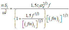(1)

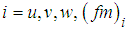where is the dimensionless frequency of the neutral spectral peak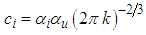, and , , and for andcomponents, respectively. The dimensionless frequency is and the dimensionless dissipation rate is obtained by

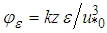(2)

where is the mean turbulent kinetic energy dissipation, is the von Kármán constant, and is the surface friction velocity [2]. The local friction velocity for a neutral PBL is

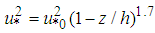(3)

according [1], where is the depth of the neutral planetary boundary layer and it could be obtained by

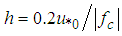(4)

and is the Coriolis parameter.

The peak frequencies and characterizing the energy-containing eddies, can be calculated by the expression

(5)

where is the frequency of the spectral peak in the surface, are constants specified from the Blackadar mixing length hypothesis and is the height above the surface.

3. Wind Tunnel Data Description

Laboratory data used for this analysis were obtained from two wind tunnels at the Universidad Nacional del Nordeste (UNNE), Argentina. One of these, the larger called Jacek P. Gorecki wind tunnel (TVG), has a test section of 2,4 m × 1,8 m (cross-section) and 22,8 m long. The other wind tunnel, the smaller (TV2), is also an open circuit with dimensions 4,45 m × 0,48 m × 0,48 m (length, height, width).

In TVG wind tunnel, the atmospheric surface-layer was simulated using the Counihan method, and employing roughness elements and mixing devices [3]. Measurements on a full-depth Counihan simulation [4] with velocity distributions corresponding to a class III terrain were accomplished. According to Argentine Standards CIRSOC 102 [5], this type of terrain is designed as “ground covered by several closely spaced obstacles in forest, industrial or urban zone”. The mean height of the obstacles is considered to be about 10 m, while the boundary layer thickness is 420 m. The boundary layer thickness in TVG wind tunnel was = 1200 mm and measurements were performed at height = 170 mm. The average wind velocity of the time series employed in this analysis was 14,86 m/s.

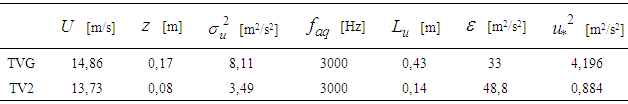
In the TV2 wind tunnel, a simulation of natural wind on the atmospheric boundary layer was performed by means of the Standen method [6], with velocity distributions also corresponding to a forest, industrial or urban terrain. A part-depth simulation with a boundary layer thickness of = 350 mm was obtained by means of spires and roughness elements and measurements were made at height = 80 mm. The mean wind velocity corresponding to TV2 measurement is 13,73 m/s.

Wind tunnel measurements were made using a hot-wire anemometer connected to a data acquisition system. Data was obtained with acquisition frequency of 3000 Hz and the anemometric signal previously was filtered by a low-pass filter set at 1000 Hz. Each time series registered in the wind tunnels consisted of 120.000 points (TVG) and 90.000 points (TV2).

Table 1 shows wind data characteristics of the time series used in this analysis; mean velocity the variance of longitudinal velocity fluctuations sample rate and the longitudinal integral length . Velocity fluctuations of and were obtained from atmospheric data. The longitudinal component was only measured by the one-channel hot-wire anemometer in the laboratory experiments. The local friction velocity was experimentally obtained for laboratory measurements and was calculated with the expression for atmospheric data. The value was adopted considering an opened area. The mean turbulent kinetic energy dissipation was determined by the fit of the structure function (four-fifths law) in the inertial range.

Table 1. Wind data characteristics

4. Results

The spectra of the longitudinal component u corresponding to laboratory measurements are shown in Figure 1. One measurement on each wind tunnel is analyzed being possible to perform controlled and repeatable laboratory measurements. It is clearly defined the inertial region (-5/3 slope), but the frequency narrow is greater for the TVG wind tunnel measurement. The low-pass filter effect is perceived at the frequency of 1000 Hz where the high frequency components are removed.

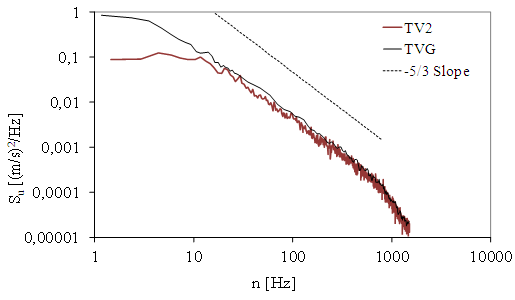Figure 1. Spectra of the longitudinal velocity fluctuations u for TV2 and TVG wind tunnel series

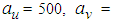
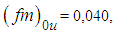
The spectral model developed by Degrazia et al. (Eq. 1) is defined using the parameters , the dimensionless dissipation rate, the local friction velocity, and the frequencies of the neutral spectral peak . The dimensionless frequencies of the neutral spectral peak were defined according [1] with and The peak frequencies in the surface are and These estimated values of the spectral peak frequencies were obtained from the north wind phenomenon in southern Brazil and they are in fair agreement with the values obtained from the data measured in Kansas experiments. The expression given by Degrazia depends on each measurement due to parameter then the comparison of dimensionless spectra should be done individually. For wind tunnel measurements, peak frequencies were directly obtained from the dimensionless spectral density functions.

Observing Fig 2 it can be seen that the mathematical formulation as provided by the Eq. (1) fits very well the spectral curves generated from the wind tunnel data. There is a good agreement between the spectral model (Eq. 1), obtained from atmospheric wind data, in the entire frequency range up to the cut-off frequency of the low-pass filter. This result is good news since that the spectral model (Eq. 1) was completely constructed from atmospheric data. This analogy between wind tunnel and wind atmospheric data allows to establish a relationship between tunnel and atmospheric spatial/temporal scales. These results guarantee that controlled studies, accomplished in wind tunnel, can be reproduce wind data observed in natural atmospheric environments.

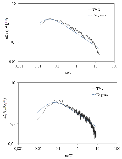Figure 2. Comparisons of dimensionless spectra corresponding to TVG and TV2 series with Degrazia et al. mode (the spectral model is defined for neutral atmospheric condition)

5. Conclusions

In the present paper, spectra measured from wind tunnel data are compared with a mathematical formulation that represents observed atmospheric neutral spectra. The analysis shows that there is a very good agreement between both spectra for the whole turbulent frequency interval. This result is important considering the fact that the spectral model was developed employing only turbulent parameters observed in the atmospheric boundary layer. This similarity between wind tunnel and atmospheric data provides a new possibility to obtain relationships between wind tunnel and atmospheric turbulent variables. As a consequence, the results obtained in the present study, corroborate the assumption that filtered turbulent variables, measured in wind tunnel, can simulate real wind data measured in atmosphere.

ACKNOWLEDGEMENTS

The authors are gratefully indebted to CNPq (Conselho Nacional de Desenvolvimento Científico e Tecnológico, Brasil) for the financial support of this work and Facultad de Ingeniería and Secretaría General de Ciencia y Técnica, UNNE (Universidad Nacional del Nordeste, Argentina).