Marcelo Coleto Rola1, Rodrigo Martins Dorado1, Marcelo Romero de Moraes2, Bardo Bodmann1
1Mechanical Engineering Graduate Program (PROMEC), Federal University of Rio Grande do Sul – UFRGS, Brazil
2Energy Engineering Graduate Program, Federal University of Pampa – UNIPAMPA, Bagé/RS, Avenida Maria Anunciação Gomes de Godoy, Brazil
Correspondence to: Marcelo Coleto Rola, Mechanical Engineering Graduate Program (PROMEC), Federal University of Rio Grande do Sul – UFRGS, Brazil.
| Email: |  |
Copyright © 2016 Scientific & Academic Publishing. All Rights Reserved.
This work is licensed under the Creative Commons Attribution International License (CC BY).
http://creativecommons.org/licenses/by/4.0/

Abstract
The study and monitoring of air quality is a problematic faced especially in large population and industrial centers. Regions around coal-fired thermoelectric power plants suffer with pollution caused by combustion processes. Currently in Brazil, enterprises that produces any kind of atmospheric pollution, must follow the normative imposed by National Environment Council (CONAMA), that is, the Brazilian regulator agency, that based on the National Air Quality Program (PRONAR), establishes the concepts of primary and secondary air quality standards. In this context, the aim of this work was evaluate the air quality in the region of the Thermal Power Plant President Médici (UTPM), in the period of two days, using the models Weather Research and Forecasting, California Meteorological Model and California Puff Model (WRF/CALMET/CALPUFF) to simulate the pollutants dispersion of SO2 (sulphur dioxide) and PM10 (particulate material 10 µm) in the atmosphere. As tools for meteorological prediction we employed the WRF models (version 3.7) and CALMET (version 6). The CALPUFF model (version 6) was used to simulate the pollutants dispersion in the atmosphere. The atmospheric pollutant concentrations simulated were compared with the results of Industrial Source Complex Model - Short Term version 3 (ISCST3) and with the values stipulated by the responsible environmental agency, keeping all within allowable standards during the two simulated days. Comparing the results of the concentrations of both pollutants to the values recorded by the air quality monitoring station, in the first simulation day the model underestimated the amount recorded by a factor of three and in the second simulation day the model presented the same value registered by the station.
Keywords:
Air quality, Pollutant dispersion, Numerical simulation, WRF/Calpuff/Calmet modelling systems
Cite this paper: Marcelo Coleto Rola, Rodrigo Martins Dorado, Marcelo Romero de Moraes, Bardo Bodmann, Air Quality Assessment and Dispersion of Pollutants in the Region of the Thermoelectric Plant President Médici Using WRF/CALMET/CALPUFF Models, American Journal of Environmental Engineering, Vol. 6 No. 4A, 2016, pp. 143-155. doi: 10.5923/s.ajee.201601.21.
1. Introduction
The city of Candiota, located in the state of the Rio Grande Do Sul (RS), has the biggest open cast coal mine of Brazil and is increasing its importance in the production of electrical energy derived from the burning of this mineral. The Thermoelectric Plant President Médici (UTPM), located near the mine, uses coal to generate electricity and currently has an installed capacity of about 796 MW. Furthermore, two other plants with capacity of 680 MW and 600 MW, respectively, are in the phase of installation in the region. Consequently, the air quality in this region will be affected due to the increase amount of coal burned, resulting in a larger fraction of pollutants emitted into the atmosphere.Air quality can be defined as the product interaction of a complex set of factors, among which stand out the magnitude of emissions, topography and weather conditions in the region, favorable or not to dispersion of pollutants [1]. In UTPM and other enterprises that use the combustion process, atmospheric emissions are characterized by gas and total suspended particles (TSP). An atmospheric pollutant can be considered as any substance present in the air, at high enough concentrations to cause measurable and harmful effects on humans, inappropriate and offensive to health, harmful to welfare, fauna, flora, and materials [2].Studies on air quality have been an important tool in this context, making it possible to evaluate and administer the volume of pollutants issued through control of combustion process. A better understanding of these processes can lead to a more suitable control over the management of air quality, because in past times the installation of an industry did not considered the meteorological characteristics of a site [3]. The complexity of the terrain is important to define parameters in the mathematical modeling of pollutants, because this factor may cause significant changes in the direction/wind speed and turbulence [4]. Based on these affirmations it is understood that certain localities may be completely inadequate for installation of a pollution source, but a previous study can indicate this inviability.The context of computational modeling has been widely applied in cases involving the behavior of dispersion of pollutants in the atmosphere. The models AERMIC Dispersion Model (AERMOD), California Meteorological Model (CALMET) and California Puff Model (CALPUFF), e.g., are certificated software and recommended by environmental agencies for studies of dispersion of pollutants [14].Many plants employ these programs to control its generation capacity, in order not to exceed the emission limits permitted by law. Moreover, it is possible to diagnose the quality of air, checking if concentrations of air pollutants emitted are within standards established by responsible environmental agencies.
1.1. Main Objective
The main objective of this study was to evaluate, during the period of two days (01/19/2003 and 01/20/2003), air quality in the region of UTPM through the results obtained from numerical simulations of dispersion of pollutants, using WRF/CALMET/CALPUFFF models.
1.2. Specific Objectives
The specific objectives are: (i) compare the simulated concentrations of sulfur dioxide (SO2) and particulate matter 10 micrometers (PM10) pollutants with values registered from monitoring stations of air quality and the Industrial Source Complex Model - Short Term version 3 (ISCST3); (ii) verify if SO2 and PM10 concentrations (simulated and registered) are within the limits allowed by the responsible environmental agency (CONAMA); (iii) evaluate the effectiveness of models used in this work; (iv) Graphic presentation of geophysical data from the study area.
2. Background
2.1. Air Pollution Process
The air pollution process can be explained as the launch of gases and particles (pollutants) into the atmosphere through mobile and stationary sources. These pollutants mixed with atmospheric gases may generate other kinds of pollutants by chemical process, which are detected by fauna, flora, people, air quality stations, etc. In urban areas, the population exposure to atmospheric pollutants is a complex parameter to evaluate, because of different air qualities of indoor and outdoor ambients frequented by people during the day [13].
2.2. Classification of Pollutants
Air pollutants are classified into two major groups: primary and secondary [2]. Primary pollutants are those emitted directly by sources and those derived from primary pollutants through transformation and photochemical reactions are called secondary pollutants [1].As examples of primary pollutants can be mentioned sulfur dioxide (SO2), hydrogen sulphide (H2S), nitrogen oxides (NOx), ammonia (NH3), carbon monoxide (CO), carbon dioxide (CO2), methane (CH4), soot and aldehydes [16]. The primary pollutants after their emission in the atmosphere are subjected to complex transport procedures, combination and chemical change, giving rise to a variable distribution, in time and space, of their concentrations in the atmosphere [17].Hydrogen peroxide (H2O2), sulphuric acid (H2SO4), nitric acid (HNO3), sulfur trioxide (SO3), nitrates (NO3-), sulphates (SO4-2) and ozone (O3) are examples of secondary pollutants [16]. In summary, distributions of pollutant concentrations in the atmosphere are subject to emission and weather conditions, causing some pollutants are led to large tracts before they reach ground level [17].
2.3. Air Quality
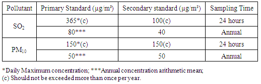
The diagnostic of air quality is measured by the magnitude of the emissions that are released, transported and diluted in the atmosphere, thereby determining the quality of the region studied [1]. In Brazil, the National Environmental Council (CONAMA) is the agency responsible for providing air quality standards established by PRONAR (National Program for Air Quality Control). The Council classified air quality standards as primary and secondary [18]: • Primary air quality standard: are those related to pollutant concentrations which if surpassed may be hazardous to human health and may be seen as maximum tolerable atmospheric pollution levels and are grouped into short and medium term standards. • Secondary air quality standards: are those related to air pollution concentrations that are not considering as being below the point when they can be hazardous to human health and well being as well as subjecting fauna and flora to minimal hazards and the environment in general, may be seen as desired levels of pollutant concentrations and are grouped into long term standards.The national air quality standard with all pollutants and its allowed concentrations is disposed in reference [18]. Table 1 shows the primary and secondary concentration standards for SO2 and PM10 pollutants.Table 1. National standards of air quality [18]
 |
| |
|
2.4. WRF/CALMET/CALPUFF Models
CALMETThe CALMET is a weather model that develops wind and temperature fields in a three-dimensional mesh in a region determined by the user. In this module is included a diagnostic wind field generator containing objective analysis and parameterized treatments of slope flows, kinematic terrain effects, terrain blocking effects, and a divergence minimization procedure, and a micro meteorological model for over-land and over-water boundary layers [13].In CALMET model are added meteorological data recorded by observation towers or in absence thereof, can be inserted meteorological data developed by forecasting models, e.g. the Weather Research and Forecasting (WRF) model. In this study, meteorological data for two-day study were obtained from WRF model, described as a next-generation mesoscale numerical weather prediction system designed for both atmospheric research and operational forecasting needs [19]. PRTMETThe Meteorological Display Program (PRTMET) is a post-processor intended to aid in the analysis of the CALMET output data base by allowing the user to display selected portions of the meteorological data, such as wind speed and direction, temperature, atmospheric pressure, humidity, among others [12].CALPUFFThe CALPUFF is a non-steady-state Lagrangian Gaussian puff model, used to simulate the phenomenon of pollutants dispersion and also for a wide variety of applications, such as modeling studies of air quality, environmental impact study, among others [13]. The configuration of CALPUFF is based on emission sources data, receptors, geophysical characterization and weather of the region, processing interval and parameters control for the simulation of dispersion [20].CALPOSTThe California Post Processing (CALPOST) performs processing of concentration data and deposition flow (dry and / or wet) contained in the output files of CALPUFF, the CALPUFF.DAT [13].
3. Methodology
3.1. Study Area
The region of Candiota, where the UTPM is operated is localized in the southwest of Rio Grande do Sul state with geographical coordinates 54º10'58"/53º18'35" West longitude and 31º17'35"/31º02'41" South latitude, distant from the capital Porto Alegre by about 420 km. It is located near Aceguá, Bagé, Candiota, Herval, Hulha Negra, Pedras Altas and Pinheiro Machado (Figure 1) [4]. Candiota hosts the biggest mineral coal mine of Brazil, administrated by the Company Riograndense of Mining (CRM). The coal reserves are 1 billion tons that can be mined open cast, at depths up to 50 meters [5].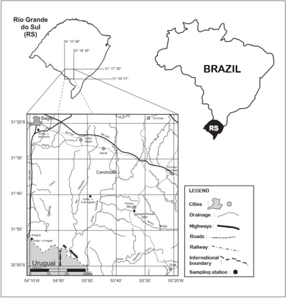 | Figure 1. Location of Candiota city [4] |
The region presents climate type CFA (subtropical climate with rainfall throughout the year, according to classification of Von Koepen [21]) and between 1961 and 1990 recorded an average rainfall of 1,465 mm, well distributed during the year with an annual average temperature of 18 °C, according to the climatological data for the weather station near the city of Bagé [4]. From December to February are recorded maximum temperatures and in the months of June and July the minimum temperatures [7].In 2003, year of interest of this study, the plant had an installed capacity of 446 MW and a daily consumption of coal for burning around 3.02 x 10³ tonnes [4, 5]. Highlights of the whole plant are a cooling tower, a structure in concrete peel with 124 meters diameter and 133 meters high, which aims to cool the water used to exchange heat in the condenser, and the exhaustion chimney with 150 meters high, which performs the release to the atmosphere of polluting gases produced by coal combustion [6].Figure 2 illustrates the plume dispersion of pollutants emitted by UTPM [6].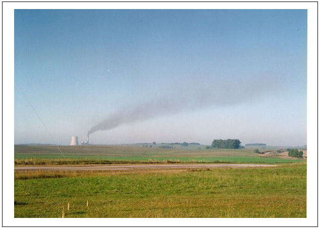 | Figure 2. Dispersion of pollutants emitted by UTPM [6] |
3.2. Concentration and Emission Data
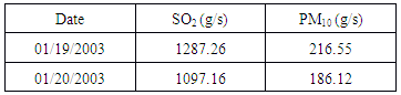
The data of air pollutants SO2 and PM10 emitted by UTPM, with reference to the days 19 and 20 January 2003, are presented in Table 2.Table 2. Daily emission of SO2 and PM10 [8]
 |
| |
|
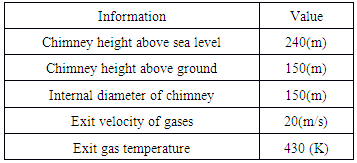
The information regarding the height and diameter of the chimney of UTPM, speed and outlet gases temperature are shown in Table 3 with their respective units of measurement.Table 3. Technical information of UTPM [8]
 |
| |
|
3.3. Pre-Processing of Geophysical Data
The pre-processing of geophysical data was performed using a CALPUFF tool, called Meteorological & Geophysical Data Preprocessors, among them are the modules: TERREL, LAND USE and MAKEGEO, where each of them has their respective functions. First of all, is necessary to get the files to configure the preprocessor of geophysical data, as follows:• Terrain Data• Land use/Land cover DataIn TERREL module were used files from the United States Geological Survey (USGS), which provides digital terrain models with a spatial resolution of approximately 1000m, all this data is distributed free of charge through the USGS website [22]. In this website, were made the downloads of elevation data of the region of UTPM and land use and cover, based on the latitude and longitude of the study region. These data have the same horizontal spatial resolution (~ 1000m), containing in this file the data of the whole continent of South America.TERRELThe terrain module (TERREL) is a land pre-processor that coordinates the assignment of elevation data from multiple databases scanned with a computational mesh specified by the user [13].In the module a square mesh of 50 km was created, with 2500 cells, horizontal spacing of 1000 meters and defined origin point in cartesian coordinates. For the region of study the projection chosen was Universal Transverse Mercator (UTM) Zone 22 and southern hemisphere, using the Datum of World Geodetic System (WSG-84), which relates to a reference ellipsoid of geocentric origin.After configured the geographic data of the study area the file with the terrain data is added. In sequence, TERREL is run, generating the output files with all information relating to the terrain.The files generated are of type .dat, .lst, .grd and .sav, and with the help of the free softwares SURFER and CALVIEW, it possible to view the terrain in two and three dimensions (2D and 3D) originating in .grd file.LAND USE/LAND COVER DATAThe processing of usage and cover land data (Land Use/Land Cover) is performed by a processor called CTGPROC, that reads the data of USGS Global Dataset format and calculates the fractional land use for each grid cell in the user specified modeling domain [13].In the present module the parameters already set in TERREL are used, however one must add the reference file for land use and cover of region. The acquisition of the data entered in this module was made through Global Land Cover Characterization (GLCC), developed by the U.S. Geological Survey (USGS), the University of Nebraska and the European Comission's Joint Research Centre (JRC). After insertion of the file of terrain use and cover (sausgs2_0l.img), the CTGPROC is executed.The files generated in TERREL and CTGPROC are compiled together to form a single file containing the data of land and land use and cover, called Creator Geophysical Archive (MAKEGEO).
3.4. Configuration CALMET Model
In the CALMET module it is possible to work with forecast data (WRF), observed data (weather stations) or both types, depending on the availability of data or user's choice.During the realization of this article the meteorological data from a station located at the airport of Candiota were not presented avaliable due to the fact that station had been disabled. Therefore, meteorological data obtained from the WRF model (version 3.7) were employed, developed and made available by the Laboratory of Modeling and Computer Simulation (LMSC) of the Federal University of Pampa (UNIPAMPA) [9]. The required basic parameters were the domain size (50 km x 50 km), containing the location of the power plant in the center of the domain with UTM projection in X and Y (245,775 km x 6506.1 km) respectively, and the grid resolution had dimensions 10 km x 10 km.The CALMET configuration is based on adding the results obtained by MAKEGEO and the WRF, which form a single file containing all geophysical and meteorological information from the power plant region.The simulation period set in CALMET corresponds to the days 01/19/2003 and 01/20/2003. The simulated data of direction and wind speed and temperature will be compared with the data in reference [8], which contains the observed values of the meteorological tower measurement located in the Candiota airport, at a height of 10 meters, with geographic coordinates 31°29'43'' South latitude and 53º41'39'' West longitude.Configured all parameters, CALMET was executed, generating two files, one being the CALMET.LST, which is a simulation control file containing configuration parameters and execution results. The other file generated is CALMET.DAT, a binary file with the data resulting from the simulation with the CALMET model, which is used as input in the CALPUFF model.PRTMETThe PRTMET provides the option to collect data at different points entered in the computational mesh, creating a file named PRTTIME.DAT. Therefore, a point in the mesh where Candiota's airport is located was inserted, to perform the analysis and comparison of the simulated and real data of wind speed and direction and temperature.
3.5. Configuration CALPUFF Model
The configuration of the CALPUFF model was divided into five stages, following the order requested by the software.First Stage: geophysical data insertion, containing all the information configured in the computational mesh.Second Stage: Description of pollutants to be analyzed in the study, in this case, SO2 and PM10.Third Stage: Insert the CALMET output file, CALMET.DAT, containing all simulated weather data.Fourth Stage: Definition of source type of the study, in this case a point source. Insertion of the location data (UTM) the power plant, along with the information in Table 2 and 3.Fifth Stage: Choice of the receptor, being selected a discrete receiver located in an air quality monitoring station of UTPM called Três Lagoas in Candiota, which is located southwest of the power plant (emission source) at a distance of about 6 km, whose elevation is 215 meters above mean sea level and its geographical coordinates are 31º34'70'' South and 53º43'68'' West [10, 11]. An option to provide the values of simulated daily average concentration has been selected in the Três Lagoas station (discrete receiver) for air pollutants PM10 and SO2. After seting all parameters the CALPUFF model was executed, generating the output files: control data and verification of the simulation (CALPUFF.LST) and simulated concentrations data in specified domain (CALPUFF.DAT).
3.6. Results Processing
To perform the processing of results the CALPUFF post-processor was applied, termed CALPOST. In this case, the simulated average daily concentrations (01/19/2003 and 01/20/2003) for SO2 and PM10 are reproduced illustratively, using maps and graphics, for a better interpretation of the phenomenon.
4. Results and Discussions
This section presents the results and discussions from the simulations. Results are separated in modules, with the same format as in this works methodology.
4.1. Pre-Processing of Geophysical Data
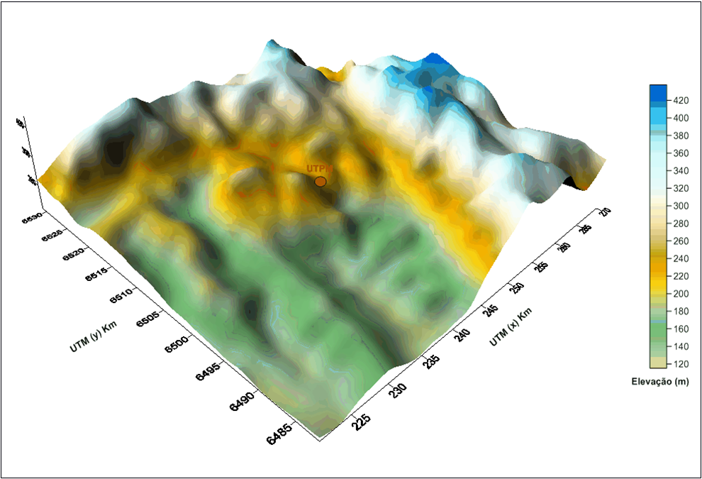
In this chapter, the results from pre-processing the geophysical data are shown and discussed.TERRELThe results from the terrain model (TERREL) is composed by four files with different extensions, however the file with the extensions GRD can be visualized graphically using free software, like SURFER or CALVIEW. Figures 3 and 4 show a two-dimensional terrain map (2D - contour lines), and a three-dimensional (3D) in UTM coordinates, respectively.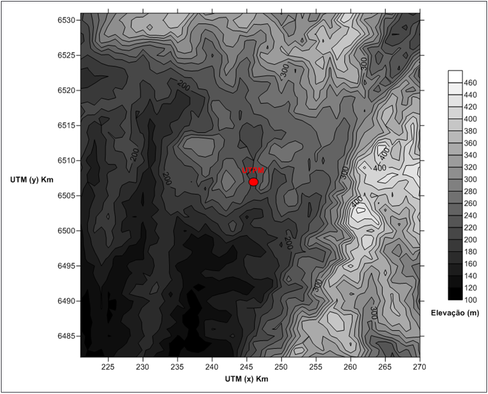 | Figure 3. Land image (2D - contour lines) |
 | Figure 4. Land image (3D) |
Regarding, the power plant surroundings, two factors are easily seen, firstly, the minimum elevation is located southwest of the power plant and has 120 meters, secondly, the maximum elevation is located east from the power plant and has approximately 420 meters. LAND USE/LAND COVER DATAThis topic shows the geophysical maps of the study area, relative to soil usage and covering, as below:• Soil usage and covering• Leaf area index• Roughness The complete classification of soil usage and covering are related to geophysical parameters, its values are available on the CALMET manual [12].Figure 5 shows the soil usage and covering for the study area in UTM coordinates.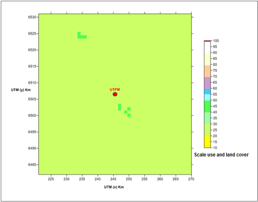 | Figure 5. Land use and land cover |
According to the CALMET manual, soil usage and covering data are classified in 10 categories and other 44 subcategories [12]. Analyzing, Fig. 5 one observes two nuances of green, a lighter one (20 to 30) and a darker one (40 to 50). The lighter green is classified as agricultural or fields/pasture, the darker is classified as forest or reforestation area.Another parameter related to vegetation is the leaf area index (LAI) shown in Figure 6. The LAI is defined as leaf area index of a population of plants and ground area occupied by it.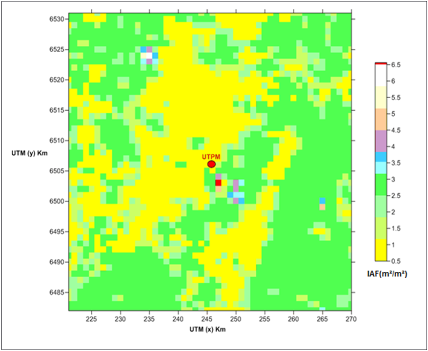 | Figure 6. Image of leaf area index (m²/m²) |
The vegetated leaf area index is based on the previously classification of soil usage and covering [12]. Pasture and low height vegetation are present in a higher amount, due to its agricultural use. Figure 7 presents the roughness for the study area.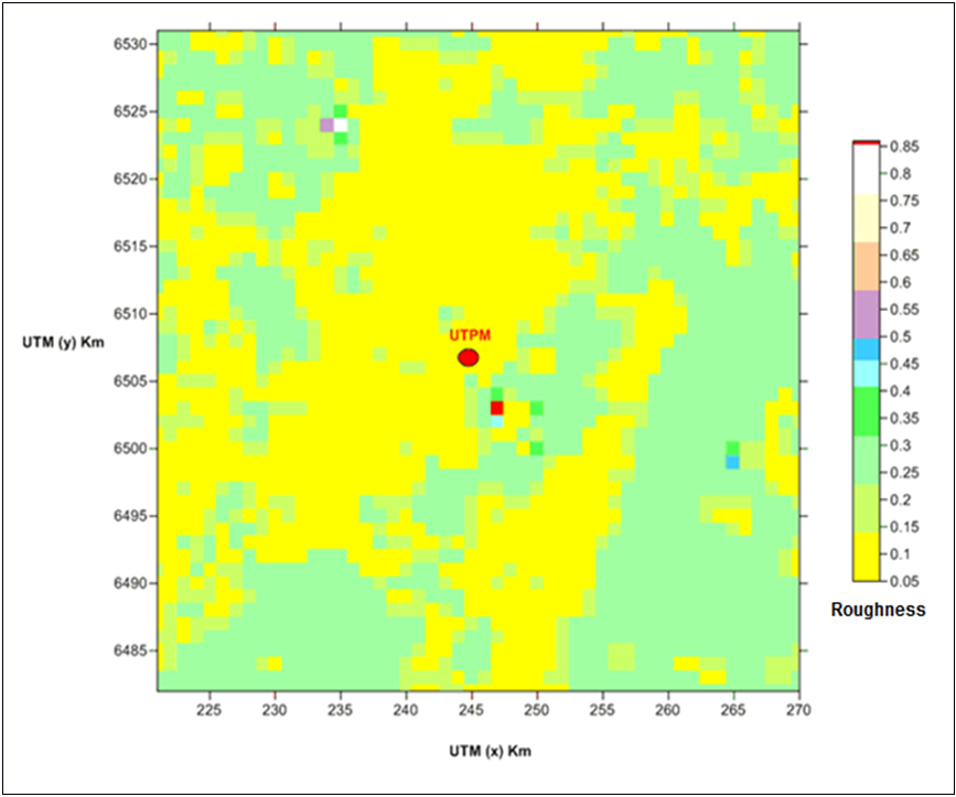 | Figure 7. Surface roughness image |
The terrain roughness image (Figure 7) its seen the predominance of pasture, in yellow, as well as agricultural areas in green, southeast from the UTPM there is a small portion of forest.All results obtained from the soil usage and covering are relevant factors on how the wind blows, changing its speed and direction, and their consequences on the dispersion process of pollutants.
4.2. CALMET
The following results describe the analysis of the meteorological conditions, simulated in the CALMET model from January 19, 2003 to January 20, 2003, which are compared and discussed with the data measured by the automatic weather station installed at the Candiota airport [8]. Figures 8 and 9 show the comparison between the real and simulated data.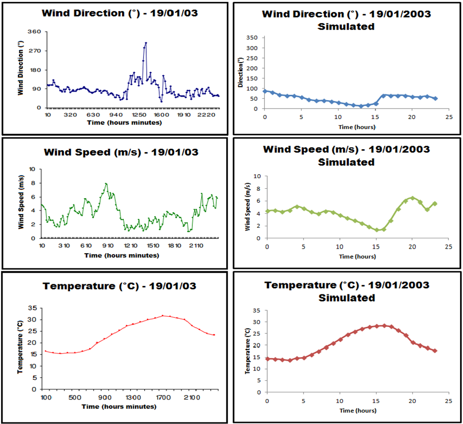 | Figure 8. Metereological results from January 19, 2003 |
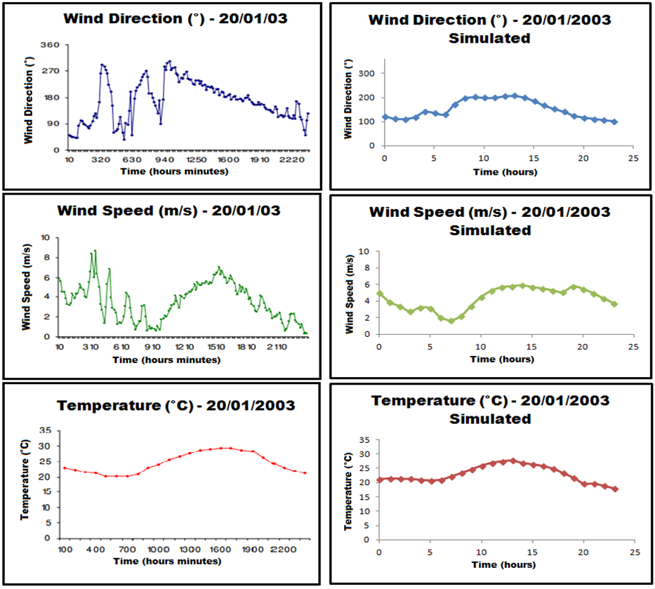 | Figure 9. Meteorological results from January 20, 2003 |
Comparing both wind direction data (Figure 8), one sees that there is a reasonable agreement between the simulated and real data, with most part the day around 60º. There is an inversion of the direction between the time frame of 11AM to 4PM in the observed wind directions, varying from 50º to 330º. In contrast, this effect is not reproduced in simulated data.By verifying the wind velocity between both graphics (observed and simulated), a similarity between the mean values is observed, around 4 m/s.The wind velocity and turbulence are considered the most important factors for the dispersion phenomenon, because as they intensify, the contaminants are dispersed more easily and, thus, their concentration decrease. Among the analyzed data, the most similar are the air temperature (see Figure 8).On January 20, 2003, the verification of the wind direction data (measured and simulated) presented similar mean values, point to 160º most of the day. The observed wind direction data pointed to significant variations in the wind direction in the time frame from 2 to 10 AM and then a linear decrease. The CALMET simulated wind direction data ranged from 100º to 210º, with a similar behavior to the observed data after 11AM.Comparing the wind velocities, one observes a similarity between the mean values, around 4 m/s. The measured data range from approximately 1 to 9 m/s, with the higher variance in the period from 3 to 9 AM. On the other hand, the simulated wind velocity data range from 1 to 6 m/s in the time frame of 8 AM to 2 PM.Once again, the air temperature graphics present the most similar behavior, when confronted to the wind direction and wind velocity. By confronting the observed and simulated data for both days, it was found that the meteorological simulated model possess similar mean behaviors to the observed data, for the most part, being possible to utilize it as input for the CALPUFF module. The difference between measured and simulated data is that the simulated values are output from the WRF. The WRF employs a computational mesh around the earth and utilizes an interpolation method to create the data based on the weather stations data, adding a built-in error and leading to a variation between both data.
4.3. CALPUFF e CALPOST
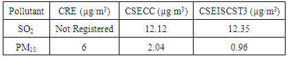
The simulated results for the daily concentrations of SO2 and PM10 were compared to the data observed by the air quality monitoring station (Três Lagoas) and to the model ISCST3 [8], as shown in Tables 4 and 5.Table 4. Observed and simulated data of SO2 e MP (PM10) (µg/m3) in the Três Lagoas station for January 19, 2003. 24h average values
 |
| |
|
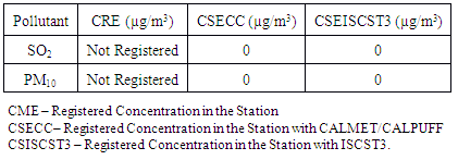
Table 5. Observed and simulated data of SO2 e MP (PM10) (µg/m3) in the Três Lagoas station for January 20, 2003. 24h average values
 |
| |
|
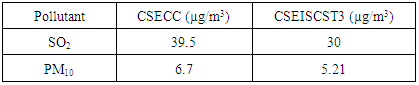
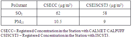
On January 19, 2003, it occurred that the CALMET/CALPUFF results for the pollutant PM10 showed a concentration three times smaller when compared to the results observed by the station, but, when compared to the ISCST3, the latter showed double the accuracy to the observed results. There was no registered values for the concentration of SO2 for this day, but both models presented strikingly similar results.On January 20, 2003, the simulated values for the concentrations of pollutants SO2 and PM10, with the CALMET/CALPUFF model, was 0 µg/m³, which was the same result found by the use of the ISCST3 model. One explanation for the values found this day is that, based on the concentration maps, the air quality measurement station is out of the wind direction field, thus not finding any pollutants in the Três Lagoas station region. In tables 6 and 7, the maximum simulated pollutants concentration in both days are described.Table 6. Maximum concentration of pollutants SO2 and PM10 (µg/m3) for January 19, 2003
 |
| |
|
Table 7. Maximum concentration of pollutants SO2 and PM10 (µg/m3) for January 20, 2003
 |
| |
|
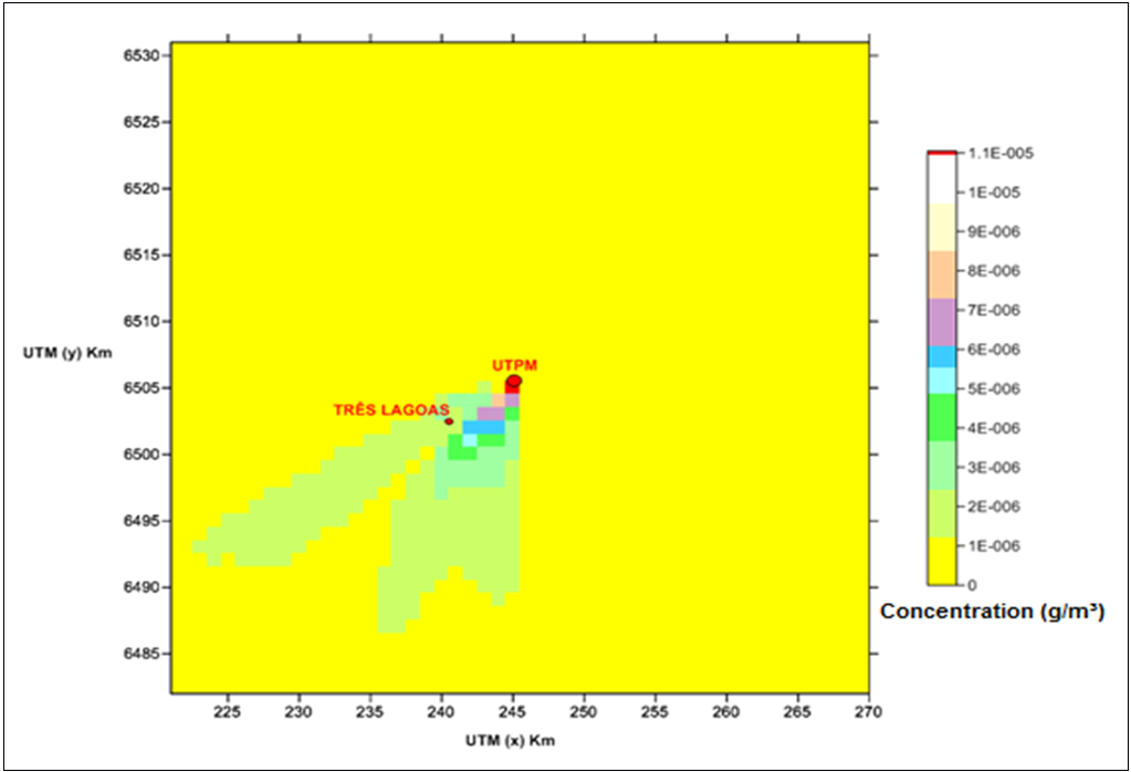
The CALPUFF post-processor software, CALPOST, generated the SO2 and PM10 concentration maps (m/m³). The maps are shown in Figs. 10 and 11, for January 19, 2003 and in Figs. 12 and 13 for January 20, 2003, respectively. In addition, the figures illustrate the positioning of UTPM and the air quality measurement station (Três Lagoas).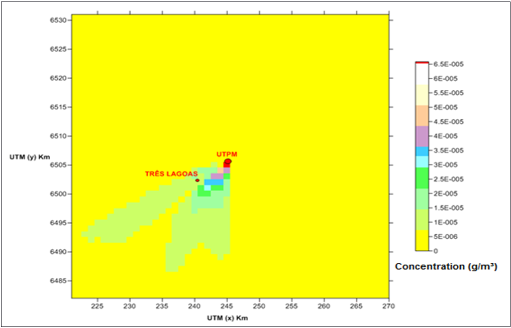 | Figure 10. SO2 concentration field (g/m³) – January 19, 2003 |
 | Figure 11. PM10 concentration field (g/m³) – January 19, 2003 |
 | Figure 12. SO2 concentration field (g/m³) – January 20, 2003 |
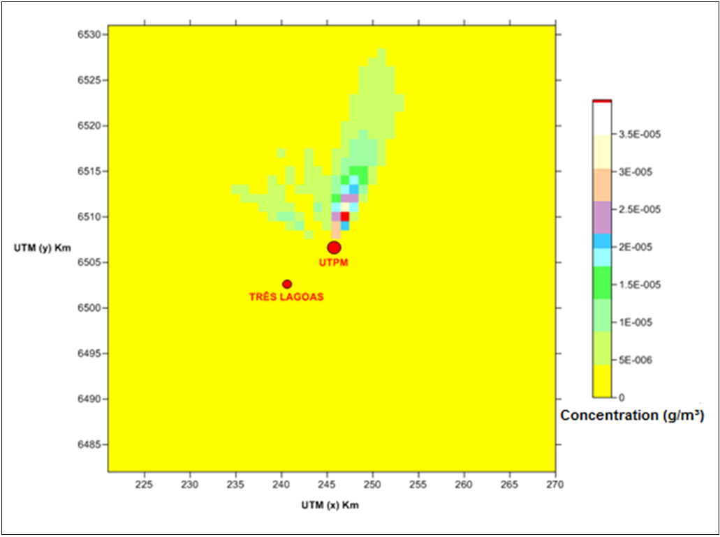 | Figure 13. PM10 concentration field (g/m³) – January 20, 2003 |
The maximum concentration values are found in the location of the power plant, as expected, since the dispersion phenomenon started as the pollutants were launched into the atmosphere. By assessing the SO2 mass concentration maps for January 19 and 20, 2003, it is worth mentioning that the highest pollutant concentration occurred on January 19, around 62 µg/m³. For January 20, the maximum concentration value was of 39.5 µg/m³. Comparing the results obtained on the models CALMET/CALPUFF and ISCST3, it was observed that the method employed in this study presented higher maximum concentration values for the pollutants.
5. Conclusions
The present work was focused on the evaluation of the air quality through numerical simulation of pollutant dispersion (SO2 and PM10) at the UTPM region, employing the models WRF/CALMET/CALPUFF. Two hypothesis were assumed for the “Non Registered” concentrations. The first suggested that the concentration was too low and the equipment did not registered any concentration. The other hypothesis was that the equipment was defective.By comparing the WRF/CALMET/CALPUFF and ISCST3 results, one concludes that both presented distinct concentration values for PM10 on January 19, 2003, while presenting similar concentrations for January 20, 2003. A probable explanation for the incoherence of the results for January 19 is that the meteorological data generated by WRF/CALMET showed different values when compared to those registered by the weather station for some period of the day, thus generating a disparity between the observed and simulated concentration data. For SO2, similar results were obtained for both simulated days.An asset in this work was the usage of meteorological data simulated with WRF, applying them as input data for the CALMET/CALPUFF models. On the other hand, the ISCST3 model utilized the observed meteorological data, which added a higher accuracy in the pollutant dispersion data.After analyzing the data from the air quality monitoring station and the data simulated with the model WRF/CALMET/CALPUFF, one concludes that the simulated values underestimate the observed values. Still, when compared to similar works in the literature (described in the references of this work), they show a similar error, demonstrating the efficacy of the employed method.By confronting the simulated concentrations of SO2 and PM10 with the air quality standards stipulated by CONAMA, one finds that these concentrations are lower than the primary and secondary standards in both days, thus being admissible by the air quality standards.Finally, the results presented in this work employing the models WRF/CALMET/CALPUFF were satisfactory, since they presented superior results when compared to the model utilized by the power plant at the time (ISCST3), showing a higher accuracy with the measurements observed in the monitoring stations and allowing a better air quality analysis.
ACKNOWLEDGEMENTS
The authors thank CNPq (Conselho Nacional de Desenvolvimento Científico e Tecnológico) for the financial support of this work.
References
| [1] | Ministry of the Environment (MMA) (MMA): Ar Quality. Homepage on MMA. [Online]. Available: http://www.mma.gov.br/cidades-sustentaveis/qualidade-do-ar. |
| [2] | J. H. Seinfeld. Atmospheric Chemistry and Physics of Air Polution. New York: John Wiley, 1986. (Reprinted, 1998). |
| [3] | M. R. Moraes. Ferramenta para a Previsão de Vento e Dispersão de Poluentes na Microescala Atmosférica. M. Eng. thesis, Graduate Program in Mechanical Engineering, Santa Catarina, Brazil. 2004. |
| [4] | C. F. Braga; E. C. Teixeira, R. C. M. Alves. “Study of atmospheric aerosols and application of numerical models,” Química Nova, vol.27, n°4, São Paulo July/Aug. 2004. |
| [5] | Company Riograndense of Mining (CRM): Candiota's Mine [Online]. Available: http://www.crm.rs.gov.br/conteudo/858 /?Mina-de-Candiota#.V7BnC_krLIU. |
| [6] | ELETROBRÁS/CGTEE: Candiota's Unit (2013). [Online]. Available: http://www.cgtee.gov.br/sitenovo/index.php. |
| [7] | National Department of Meteorology (Brazil), 1992, p. 84. |
| [8] | A. S. Nedel. Aplicação de um Modelo de Dispersão de Poluentes na Região de Candiota-RS e sua Relação com as Condições Meteorológicas. M. Eng. thesis, Program in Remote Sensing, Porto Alegre, Brazil. Oct. 2003. |
| [9] | Modeling and Computer Simulation Laboratory (LMSC) of the Federal University of Pampa (UNIPAMPA). [Online]. Available: http://lmsc.bage.unipampa.edu.br/. |
| [10] | C. F. Braga. Estudo dos Compostos Inorgânicos em Partículas Atmosféricas da Região de Candiota-RS Utilizando a Técnica Pixe. Catholic Pontifical University (PUC), Porto Alegre, Brazil, 2002. |
| [11] | MORAES, O.L.L. Um Estudo Observacional das Circulações Atmosféricas e das Propriedades Difusas na Região de Candiota. Federal University of Santa Maria (UFSM), Santa Maria, Brazil, 1996. |
| [12] | A User’s Guide the CALMET Meteorological Model. (2000). [Online]. Available: http://www.src.com/calpuff/ downloadCALMETUsersGuide.pdf. |
| [13] | Atmospheric Study Group of TRC (ASG). CALPUFF Modeling System. Version 6. (2011). [Online]. Available: <http://www.src.com/calpuff/download/ CALPUFF_Version6_ UserInstructions.pdf. |
| [14] | Preferred/Recommended Models. 2016. [Online]. Available: https://www3.epa.gov/scram001/dispersion_prefrec.htm. |
| [15] | R.W. Boube, D. L. Fox, and D. B. Turner., Fundamentals of Air Pollution. 3 ed. New York: Academic Press, 1994. |
| [16] | T. J. Lyons and W. D. Scott., Principles of Air Pollution Meteorology. London: Belhaven Press, 1990. |
| [17] | D. M. Elson., Air Pollution: Causes, Effect and Control Policies. New York: Basil Blackewll, 1989. |
| [18] | CONAMA, National Environment Council, Resolution n° 03 of 28 june 1990, 4ª Ed. Brasília, 1992. |
| [19] | The Weather Research & Forecasting Model. 2016. [Online]. Available: http://www.wrf-model.org/index.php. |
| [20] | L. A. Soares, L. N. Ramaldes., Estudo Comparativo dos Modelos de Dispersão Atmosférica - Calpuff e Aermod - Através da Análise da Qualidade do Ar na Região Metropolitana da Grande Vitória. Federal University of Espirito Santo, Vitória, Brazil, 2012. |
| [21] | W. Köppen., Climatologia. Ciudad de México: Fondo de Cultura Económica, 1948. |
| [22] | United States Geological Survery (USGS). [Online]. Available: https://www.usgs.gov/ |

 Abstract
 Reference
 Full-Text PDF
 Full-text HTML