1. Introduction

Quality assurance and quality control are fundamental procedures when dealing with data analysis. This is particularly true in meteorological observations, where the measured variables are almost always hampered by imprecision and errors. In micrometeorological observations, in addition to that, the high-quality data necessary due to the small differences and gradients involved are especially troubling [1].

According to [2], time series can be influenced by instrumentation problems, like malfunctioning or external influences on the sensor, flux sampling problems, and physically plausible —but unusual— situations. In that way, quality control procedures must identify and correct these data when possible. However, methods specifically designed for micrometeorological conditions and high temporal resolution of the data are rare [1]: correspondingly, in most cases the steps of the quality control procedures are subjective and chosen according to the researcher.

The increasing use of electronic sensors and computerized storage has introduced an abundance of new problems [1], of which the most common is the presence of spikes in time series. Spikes can be caused by random electronic peaks in monitoring systems or by physical alteration of the measuring conditions, such as water collecting on the sonic anemometer's transducers during precipitation [2], and are typically characterized as short duration and large amplitude fluctuations [3]. If not removed from the original series, spikes can contaminate turbulent flux calculations and data statistics.

Other types of effects that can negatively alter data are missing values in the time series, dropouts (abrupt and large changes resembling discontinuities), and “freezing” or “sticky” values, all of which are cases of sensor or logger malfunction [2].

Besides detecting errors in high frequency data, quality control is essential to indicate when the time series is in accordance with the assumptions of the micrometeorological theories. One of the most important of these is stationarity, which is one of the conditions for Monin-Obukhov Similarity Theory (MOST) and the Eddy Covariance method (EC) to be valid [4]. In complement, the EC method also requires fully developed turbulence. For [5] and [3], quality control of eddy covariances should include not only tests for instrument errors and problems with the sensors, but also evaluate how closely conditions fulfill the theoretical assumptions underlying the method. Because the latter depends on meteorological conditions, eddy covariance quality control tools must be a combination of typical tests for high-resolution time series and criteria that allow examination of the turbulent conditions. According to [1], it is important to minimize all errors of the EC measuring system and to try to exclude all other erroneous influences (e.g., bad weather conditions, unsuitable underlying surface, etc.) for which the method is not defined.

Unfortunately, as mentioned before, widely accepted standardized methods for data screening do not exist yet, and these procedures are usually left for the analyst to choose. Still, in a recognition by the micrometeorological community of the importance of the issue, there are now works dealing specifically with quality control of high frequency data [1, 2, 6] and with quality control of EC measurements [3, 5-9]. These works, albeit still few in number, have now formed a basis for progress towards a more unified and more widely accepted approach to data quality control in micrometeorology.

The present work was motivated by the need to process large amounts of micrometeorological data now being produced within the context of the ATTO project [10]. While following the guidelines set forth by the aforementioned works on data quality control, we have found the need to at times expand, or adapt, those existing methodologies. Specifically, given the abundance of data produced at the ATTO site, we choose fast-to-execute tests over tests that are more elaborate but tend to have a larger runtime. This characteristic is often overlooked by quality control procedures, but is important in some cases when large amounts of data have to be processed.

In this context, the goal of this paper is to propose a set of simple data quality procedures aimed to process high frequency micrometeorological data, while introducing a few new approaches that we have found particularly useful; in addition, to validate our quality control, we apply it to a large set of experimental data measured at the ATTO site as an example. Part of these procedures were previously reported in [11] as research-in-progress, and many of the steps of the quality control reported here were applied in [12], where they were briefly summarized.

The paper is divided as follows. In Section 2 we describe the experimental site and the dataset; in Section 3 the procedures for quality control are explained in detail. Results and examples are given in Section 4. We conclude briefly in Section 5.

2. Site and Data Description

The experimental site is that of the Amazon Tall Tower Observatory (ATTO) project, located in the Amazon rain forest, approximately 150 km Northeast of the city of Manaus, Amazonas State, Brazil. The latitude and longitude coordinates are 2.144°S, 59.002°W. A detailed description of the project and the experimental site can be found in [10].

The data were measured at height of 46.46 meters during a 10-month period between March 1st and December 19th, 2013. The variables used in this analysis were the three velocity components (u, v and w in ms⁻¹) measured by a WindMaster 3D Anemometer (Gill), the virtual temperature, θ_v (°C), also measured by the WindMaster 3D Anemometer, and the CO₂ and H₂O molar densities ρ_c and ρ_v (mmol m⁻³) measured by a LI7500 (LI-COR). The acquisition frequency was 10 Hz, and the data were separated in 30-min runs, or blocks, of 18000 lines. The word ‘line’ should be understood here as a record of six simultaneous measurements of u, v, w, θ_v , ρ_v and ρ_c, but it is also a convenient reference to the text files where the data resided. A total of 13281 runs were analysed in this work.

3. Quality Control Procedures

In this section we describe each of the steps of the proposed quality control in detail. Although some steps may be well known, they have been included for completeness. Furthermore, it is important to mention that the order in which the tests are applied respects the order in which they are described here. Figure 1 presents a flowchart summarizing the steps for the quality control.

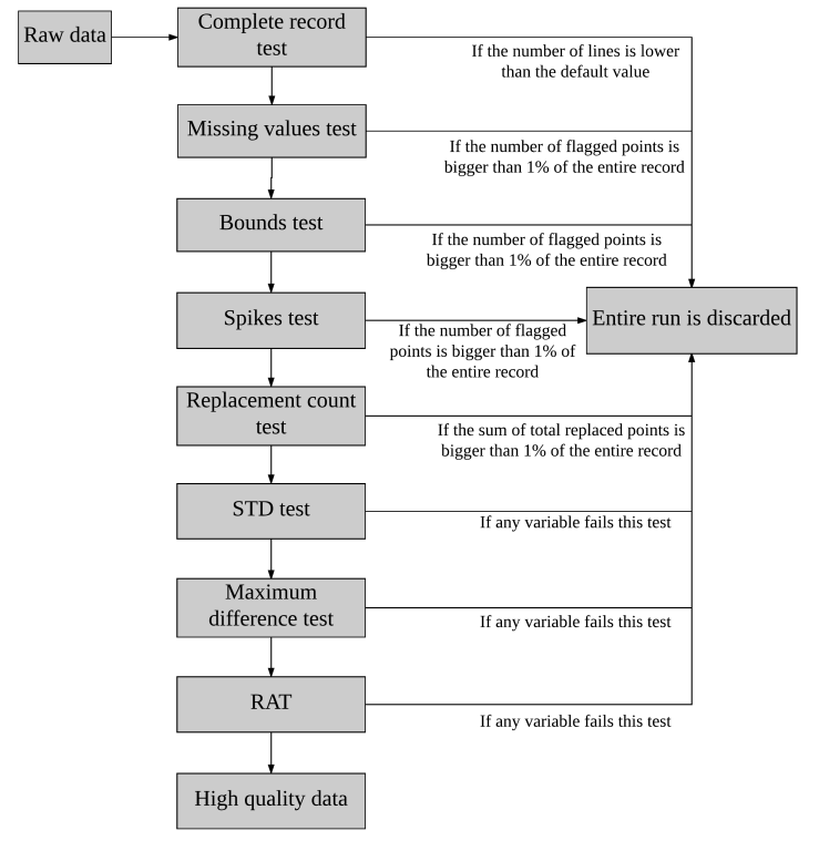Figure 1. Flowchart of the proposed quality control. Note that when any variable of the run fails a test, the entire run is discarded

3.1. Complete Record Test

First, we check if each of the runs has the correct number of lines. This test is characteristic of micrometeorological processing, since it is common for each data file to correspond to one averaging period and, ultimately, to one set of fluxes. The correct number of lines in the file depends on the total time duration of the run and on the logging frequency. In our case the number of lines (18000) corresponds to a 30-minute run with a measurement frequency of 10 Hz. Runs with different number of lines than expected may be the result of problems with the logging of data, and are discarded.

Admittedly, this may eliminate good data, and in some circumstances it might well be worth trying to recover valid data in these situations. On the other hand, as massive amounts of data need to be screened and then processed, such attention to detail quickly becomes counter-productive. This procedure, although not usually reported in the literature, is quite common. It is mentioned here for the sake of completeness.

3.2. Missing Values Test

In this test we check the presence of error flags in the data. These flags generally appear as a “NAN” flag (acronym for Not a Number) or a specific impossible or implausible value, such as −9999. In the interest of simplicity, we call them all NAN's. Whenever the number of NAN's in the series is higher than 1% of the total number of points (or 180 values), the entire run is discarded. Notice that it suffices for this to happen to a single variable in the run; again, it is possible to recover data from the other variables, but again, as the volume of data processing increases, this becomes more cumbersome. If the number is below this level, they are filled in by linear interpolation of the existent adjacent points (end points are extrapolated).

Although the accepted percentage of NAN flags is open to debate, this test is crucial for any type of dataset, since it is not uncommon for a logging system to malfunction and output data that consist mostly of error flags. Again, although this test is not often documented, it is common in practice and is included here for completeness.

3.3. Bounds Test

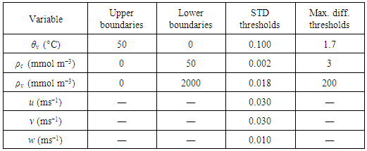
This test is well documented among quality control procedures [2, 6] and it identifies values above and below pre-defined upper and lower bounds, respectively. Detected points are replaced by linear interpolation if they are 1% or less of the total. If the number of points flagged by this test is higher than 1% the run is discarded. We define bounds for the velocity components u, v and w, the virtual temperature θ_v and molecular densities of CO₂ (ρ_c) and H₂O (ρ_v ), which are given in Table 1.

Table 1. Threshold values used in the proposed tests. The upper and lower boundaries refer to the Bounds test, the standard deviation (STD) threshold refers to the STD test and the maximum difference thresholds refer to the Maximum difference test

The bounds can and should vary from one site to another. As an example, values below 0°C are likely to be measurement errors if the sensor is placed in a tropical low-altitude environment, but are considered normal values for high latitudes. The opposite goes for high temperatures such as 40°C.

The values of the bounds have to be chosen according to the number of false positives and false negatives the researcher is willing to accept. Narrower limits have a greater chance of discarding runs with properly-measured variables (false negatives). However, it is recommended that the bounds be set at least to flag impossible values, such as negative concentrations, relative humidities greater than 100% and so on. Applying this very-conservative set of limits increases the chance of not flagging improperly-measured runs (false positives).

It is worth noting that we focus this analysis on cases where sensor diagnostic flags are not available, which are the result of internal quality tests provided by modern micrometeorological sensors [6]. However, for cases where diagnostic sensor flags are available, this test may (and should) also be applied using them to detect and replace poor quality data [6].

3.4. Spikes Test

This test is traditionally applied using a moving average across the complete run [2], while recent studies have proposed a single median over the 30-minute window alongside calculations of the median absolute deviation [6]. We propose a method that we found to be a good compromise between both, since it is considerably faster than applying a moving window with almost the same results. It is applied according to the following steps.

Initially, (i) the time series is de-trended with a linear fit and then divided into windows of 2 minutes each (1200 points in our case). Next, (ii) we calculate the median absolute deviation (MAD_n) and median for each 2-minute window, where n=1,2,…15. Running point-by-point within the 2-minute window, the point is flagged if it satisfies the condition

(1)

where the a_i’s are each point in the 2-min window (i=1,2,…,1200) and λ is a constant found by trial and error; an optimum value for our dataset is λ = 7, which is also used by [6]. The factor 0.6745 is a constant that relates the median absolute deviation to one standard deviation, assuming a gaussian distribution [6]. Moreover, (iii) if there are four or more consecutive flagged points, then they are not considered spikes and are not modified. If they appear in a maximum of three consecutive values, they are considered spikes and are linearly interpolated. Finally, (iv) if the total number of spikes after this procedure is greater than 1% (considering the complete 30-minute run), the run is discarded.

3.5. Replacement Count Test

After the three previous tests which effectively replace values and correct the data are applied (namely the Complete record, Missing values and Spikes test), we check if the sum of the total replacements made in those tests exceeds 1% of the total values in the time series. If this occurs for any variable, then the entire run is discarded.

This step makes sure that runs that passed the Complete record, Missing values and Spikes test do not have a combined number of replaced data points large enough to potentially alter significantly the statistics derived from them. Versions of this test are already used in the literature, with values of accepted percentage ranging up to 10% [6].

3.6. STD Test

According to [2], for some records with low variance (weak winds and stable conditions), the resolution of the sensor may not be fine enough to capture the fluctuations, leading to a step-ladder appearance in the data. Resolution problems also might result from a faulty instrument or data recording and processing systems [2]. Although other approaches to identify such conditions exist [2], we propose a simpler and faster approach which is done by comparing the standard deviation (STD) of each variable with pre-stipulated calibrated values (near the resolution of the sensors) in order to check the reliability of the measurements.

In this test, first (i) the trend should be removed for all variables using a two-sided moving average with a 900-point window, creating a fluctuation series (notice that the objective here is not to “extract” the turbulent fluctuations which will be used, eventually, to calculate the turbulent statistics; these fluctuations are specific to the test at hand). Next, (ii) these new series are divided in windows of 2 minutes and the standard deviation of each window is computed. Finally, (iii) the standard deviation of each window is compared to threshold values previously stipulated, whereas runs that have any 2-minute window with a standard deviation smaller than the threshold for any variable are discarded.

Although the thresholds for each variable have to be carefully chosen by trial and error, given that they are sensitive to small changes, it is reassuring that the thresholds which are eventually obtained are often close to the nominal sensor resolution. The values used in this work are presented in Table 1.

3.7. Maximum Difference Test

We propose this test to remove runs that remain non-stationary even after linear detrending. It is applied by (i) taking the fluctuations of each variable using a linear detrending procedure. Next, (ii) the absolute difference between the highest and lowest values in the moving-median of this 30-minute fluctuation is computed using a 1-minute window. Finally, (iii) runs for which this “maximum difference” is greater than a pre-defined threshold for any variable are excluded.

Threshold values were chosen empirically using visual inspection of some time series as an essential procedure. This test is applied only for the virtual temperature, ρ_c, ρ_v, and the values adopted here are presented in Table 1.

3.8. Reverse Arrangement Test

The Reverse arrangement test (RAT) is included to detect trends in data and exclude non-stationary time series that were not detected by the Maximum Difference test. According to its definition [13], from the number of observations in the series (N), the RAT calculates the number of reverse arrangements, denoted by A. Then, given a significance level (α), the acceptance range stipulated for this test is [A_N;1−α/2 < A ≤ A_N;α/2], whose values are tabulated and can be found in [13, p. 97].

To apply the RAT we divide the 18000-point time series in 50 intervals, and the mean of each of those intervals is used in the test, representing an “independent” point in the sample, for a total sample size N = 50. A 5% significance level is adopted. In terms of the RAT statistic A, the acceptance range is [495 < A ≤ 729]: for this level of significance the number of reverse arrangements A of the 50-points averaged series has to be in the range (495, 729] in order for the run to pass.

The RAT is applied after linear detrending; in fact, in our experience, only then is the RAT is effective. If the fluctuations are extracted with a block average, then it flags almost every run (because a net trend remains in the fluctuations); on the other hand, if the fluctuations are extracted with a moving mean/median, then almost no run is flagged by the RAT.

4. Results and Discussion

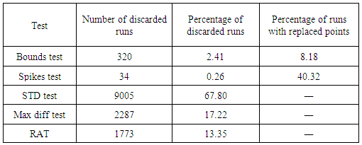
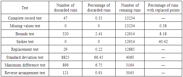
In this section we show the results for the application of the quality control procedures to our dataset along with some general remarks on its application. Although each dataset should be evaluated independently, we believe that the application of the quality control to the data obtained in our site could illustrate and serve as an example to other applications.

First of all it is important to perform a visual inspection on some of the runs of the dataset. Depending on the size of the dataset, it is impractical to view more than a small fraction of the total; however, viewing a set of runs that include both daytime and nighttime runs under different stability conditions is usually a helpful procedure. This can aid the analyst to develop a feeling about what to pay most attention to in the quality control and later to check, to the best of his/her judgement, if the discarded runs were flagged correctly.

As described in the previous sections, the parameters of each test are dependent on the experimental site and dataset, and should be found by trial and error. In our case, as already mentioned, the quality-control parameters thus found are listed in Table 1.

In order to better understand and exemplify each test, we performed two applications of our quality control procedure. The first application is designed for the illustrative purposes of this work only, while the second is the real intended application of the procedure described here.

In the first case we initially removed the runs that failed the Missing values and Complete record test, which totaled 47 runs, leaving 13234 runs. This has to be done since runs with less lines than what is expected or with too many NAN's may incorrectly fail tests such as the STD and Spikes test, producing a false count for them. Next, all runs were submitted to all remaining tests of the quality control independently. By this approach, every run passes through the Bounds, Spikes, STD, Maximum difference and Reverse arrangement test. The Replacement test was not applied in this approach because for this test to make sense, by its definition, the Missing values, Bounds and Spikes test have to be applied together, and not independently.

The results of this exercise can be seen in Table 2, where the first column shows the number of excluded runs by each method and second column shows the respective percentage of the total of runs (13281). For our dataset the standard deviation test, by itself, was responsible to exclude the majority of the original runs (almost 68%), with the variable most responsible for failing the STD test being θ_v, measured by the sonic anemometer.

Table 2. Summary of discarded runs for each test of the quality control when applied individually

After inspection, we found that the resolution of the sensor was in fact close to what is described in the manufacturer's manual. Furthermore, from all the runs discarded by this test, 61% were between 6 pm and 6 am of the following day, which indicates a low-turbulence scenario. An example of series detected by this test is shown in Figure 2-b.

Moreover, the Maximum difference and Reverse arrangement tests are responsible for the second and third most discarded runs (17.22 and 13.35%, respectively). However, as we will explain next in the second application of the quality control, most of these runs overlap and are discarded by both of them. Furthermore, although the number of runs that failed the Spikes test is small, we see that this test is important since it replaced spikes in 40.21% (5355 runs) of the original runs. Examples of runs that failed the Maximum difference and Reverse arrangement tests (respectively) are shown in Figure 2-a and 2-c.

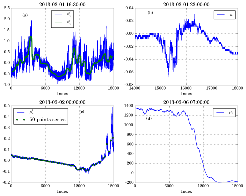Figure 2. Examples of some runs that were discarded by some tests. In panel (a) we show the fluctuations of a run that failed the Maximum difference test, along with the moving median used in the test. In (b) we show an example of a run that failed the standard deviation test. In (c) we present a run that failed the Reverse arrangement test, along with the 50-points array used for the actual application of the test. Lastly, in (d) we have a run which clearly fails the Bounds test because of the negative concentrations

In the second case all tests were applied to the dataset sequentially. Therefore, if a run fails one test, it will not be tested for the others, which is how this quality control procedure should in fact be used. The results for this application can be found in Table 3, whose rows follow the order in which the tests were applied, which can also be seen in Figure 1.

Table 3. Summary of the quality control steps when applied sequentially

To begin our analysis for the sequential application, we note the fact that although no run was discarded by the Missing values test, such a test is still important for datasets in general, since it is a simple test that can quickly detect data logger errors. Furthermore, although it did not exclude any run, 0.38% of runs had NAN’s that were interpolated and which could possibly alter results for other tests. It goes without saying that this percentage could be larger for other datasets.

The Bounds test, which is applied before the Spikes test, effectively removes many spikes already. This is an argument for applying the Bounds test before the Spikes test, since the Bounds test is simpler and far less computationally costly, which may make a significant difference in the run-time required to screen large datasets. An example of a run that fails the Bounds test is shown in Figure 2-d.

Still, the Spikes test removed spikes from approximately 40% of runs, without however being responsible for discarding any run (which means that spikes were not particularly abundant in any run). The Spikes test was also important preventing those relatively few spikes from “contaminating” the next tests in the order of application.

The STD test, when applied in sequence to the previous tests, still discards the majority of our runs. Although the discarded count for this test is high and in the majority of these cases the variable responsible for failing this run is the virtual temperature, we found by thorough visual inspection that our calibration of the STD limit for this case is accurate. Thus, for this dataset this test was crucial to identify low-turbulence runs, whose measurement suffers from insufficient sensor resolution, from passing to possible further analysis. It is outside our scope to undertake a more detailed analysis of such runs. There is an abundance of advanced techniques to deal with these situations [14-19], in which case it may well be needed to reconsider the elimination of all these runs, without further analysis, from the final dataset.

The Maximum difference test had a drop from 17.22% (when it was applied independently for all runs) to 6.75% of failed runs (when applied in sequence). Such drop is expected for tests placed last in the order of application. The Reverse arrangement test, however, decreased from excluding 13.35% of runs to only 0.91%. Since the Reverse arrangement test and the Maximum different both aim at excluding non-stationary runs, it is likely that for this test the great majority of non-stationary runs are already identified and discarded by the Maximum difference test, leaving a small number of runs that fit into the RAT characteristics.

We suggest that this analysis be done for other datasets to find whether this redundancy between the STD and RAT continues. If so, then we recommend that only one of those tests be used. According to the discard count in Table 2, the Maximum difference test is more rigorous than the RAT. However, on average, the RAT is 15% faster to run than the Maximum difference test. Thus, if the quality control has to be extremely focused on small runtimes, it should be better to use the RAT. On the other hand, if some speed can be given up for accuracy, it may be preferrable to use the Maximum difference test.

The Replacement test excluded a total of 0.22% of the runs. This count is low when compared to other tests, but may be larger for other datasets. Finally, when the quality control was applied sequentially, the number of remaining runs was 3043, corresponding to roughly 22.91% of the original number of runs. This percentage is low, with most of the runs excluded being night runs with low turbulence.

5. Conclusions

In this paper we proposed a simple quality control procedure for high frequency micrometeorological datasets. Although there exist other proposed procedures for quality control of environmental data in general [1, 2, 6], we focused on tests that can be applied fairly easily to high-frequency data, and that are computationally efficient, rather than tests that have a large runtime.

Furthermore, since our methods are specifically tailored for micrometeorological datasets, they aim mostly at improving the quality of the fluctuations. Although some of our tests may be useful for other types of applications, in that case other methods of quality control should be considered, such as a detection of non-stationarity in the means of time series and an analysis of sensor accuracy as opposed to resolution.

Our proposed procedure was applied to data collected over a tropical forest in the Amazon basin. First we applied each test independently in order to check what were the most common issues of the time series and to exemplify each test. Next we applied all tests in sequence, where runs that fail one test were excluded and not tested again.

Overall, we found that the proposed quality control was successful in removing the majority of errors and non-conformities with the micrometeorological theory that may affect datasets, such as unrealistic data values, insufficient sensor resolution and non-stationarity.

We found that in both applications the STD test was responsible for excluding the majority of runs, which can be attributed to low-turbulence periods in which the sensor is unable to properly measure because of insufficient resolution. The second most frequent problem with our dataset was non-stationarity of the time series, for which the Maximum difference test seems to be enough, although another test is proposed (namely the Reverse arrangement test) to discard runs that eventually pass the former.

The tests described here (along with additional options) were included in the quality control function of the Python tool for Micrometeorological Analysis (Pymicra), which is available at Github (https://github.com/tomchor/pymicra).

ACKNOWLEDGEMENTS

We thank the Max Planck Society and the Instituto Nacional de Pesquisas da Amazonia for continuous support. We acknowledge the support by the German Federal Ministry of Education and Research (BMBF contract 01LB1001A) and the Brazilian Ministério da Ciência, Tecnologia e Inovação (MCTI/FINEP contract 01.11.01248.00) as well as the Amazon State University (UEA), FAPEAM, LBA/INPA and SDS/CEUC/RDS-405 Uatumã.

We also would like to thank Prof. Antônio Manzi, Marta Sá, Paulo R. Teixeira and Prof. Alessandro Araújo for the datasets.