-
Paper Information
- Next Paper
- Previous Paper
- Paper Submission
-
Journal Information
- About This Journal
- Editorial Board
- Current Issue
- Archive
- Author Guidelines
- Contact Us
American Journal of Environmental Engineering
p-ISSN: 2166-4633 e-ISSN: 2166-465X
2016; 6(4A): 119-128
doi:10.5923/s.ajee.201601.18

A Review of Temperature and Emissivity Retrieval Methods: Applications and Restrictions
 Abstract
 Reference
 Full-Text PDF
 Full-text HTML
Silvia Beatriz Alves Rolim1, 2, Atilio Grondona3, Cristiano Lima Hackmann2, 4, Cristiano Rocha2
1Geosciences Institute, Federal University of Rio Grande do Sul, Porto Alegre-RS, Brazil
2Graduate Program in Remote Sensing, Federal University of Rio Grande do Sul, Porto Alegre-RS, Brazil
3Department of Engineering, College of Technology TecBrasil - Porto Alegre Unity, Porto Alegre-RS, Brazil
4Interdisciplinary Department in Science and Technology, Federal University of Rio Grande do Sul, Porto Alegre-RS, Brazil
Correspondence to: Silvia Beatriz Alves Rolim, Geosciences Institute, Federal University of Rio Grande do Sul, Porto Alegre-RS, Brazil.
| Email: |  |
Copyright © 2016 Scientific & Academic Publishing. All Rights Reserved.
This work is licensed under the Creative Commons Attribution International License (CC BY).
http://creativecommons.org/licenses/by/4.0/

Remote data coming from the Thermal InfraRed (TIR) region of electromagnetic spectrum has several applications in geology, climatology, energy balance, biological and geophysical process analysis, disaster assessment and change detection analysis. In the TIR region, the emission of the targets is dominant when compared with reflection. This radiation is a function of two unknowns – the emissivity and the temperature of the target. To study TIR, a precise retrieval of the temperature and/or emissivity from the measured radiation is necessary. This process is usually difficult due to a non-linear relationship between these two unknowns and the measured radiation. In the last 40 years, several researchers have developed approaches to generate reliable results. However, all these methods have constraints in their applications. This paper reviews the advantages and disadvantages of the main methods of temperature and emissivity separation in order to create a summary that allows the researchers to choose the most suitable method in their own application.
Keywords: Thermal Infrared, Temperature Emissivity Separation, Temperature Retrieval, Emissivity Retrieval, TIR, TES
Cite this paper: Silvia Beatriz Alves Rolim, Atilio Grondona, Cristiano Lima Hackmann, Cristiano Rocha, A Review of Temperature and Emissivity Retrieval Methods: Applications and Restrictions, American Journal of Environmental Engineering, Vol. 6 No. 4A, 2016, pp. 119-128. doi: 10.5923/s.ajee.201601.18.
Article Outline
1. Introduction
- Remote sensing was initially developed for military purposes in the mid-twentieth century, and later, for scientific research capabilities of the Earth's surface and other planets. The advantage over other similar alternatives are low cost, synoptic view and temporal resolution. Initially, the technological knowledge allowed only the study of physical and chemical properties of targets through the reflection of the incident radiation in the visible region (VIS) and shortwave infrared (SWIR) of the electromagnetic spectrum (EEM). With the advance of technology, other regions of the EEM were included in the study of Earth's surface, such as the thermal infrared (TIR). In TIR the chemical and physical properties of targets are studied through their radiation at a particular temperature. In this region, it can be assumed, under certain conditions, that the target radiation emission is inversely proportional to its reflection. In TIR, different intrinsic properties of the targets can be evaluated by their capacity to absorb and re-emit radiation that strikes it, manifest in emissivity. However, as the temperature varies, the target emissivity varies and all other intra-target relations change. This complex dynamics of relationships within the target (atomic level) propagate in a cascade effect reflecting variations in determining emissivity. The model of this problem shows that the target radiation measured by the sensor is a function of the emissivity of this target in the temperature during the measurement. From a mathematical point of view, the equations modelling this problem form an indeterminate system, where the number of measured variables exceeds the number of model equations. This problem makes it difficult the use of TIR data in the recovery of emissivity and / or the target temperature measured by radiance. The difficulty is the existence of infinite solutions in an indeterminate system.Therefore, the main point to be searched is to obtain a method, even not optimal, but with a minimum of mathematical-physical restrictions and with the result of lowest possible error.In the last 40 years some authors (Collins et al. (1999) and (2001); Hook et al. (1992); Kealy and Hook (1993); Gillespie (1985), Gillespie1 (1992); Gillespie2 (1992); Gillespie et al. (1999); Watson1 (1992) and Watson2 (1992); Schmugge et al. (1998); Coll et al (2007).; Barducci and Pipi (1996); Kahle and Alley (1992) among others) have been developing and improving methods of separation of temperature and emissivity (TES -Temperature and Emissivity Separation) for TIR. The physical value remotely measured by the sensor in TIR is the spectral radiance, defined as the radiant flux in a given direction, from a standardised surface related to unit surface area and solid angle (Siegel et al., 1982). This is valid for the entire electromagnetic spectrum. In the thermal region, one can take into account spectral emissivity, which is an index that tells how capable a material is to transform the energy that strikes it into thermal radiation. This index is related to the spectral radiance and Planck’s function for a blackbody (under the same wavelength and temperature). Planck's function is given by the following equation,
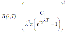 | (1) |
 is the radiation re-emitted by the blackbody,
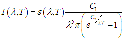
  is the wavelength (µm), T is the surface temperature (K),
 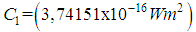 is the first radiation constant and
 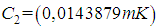 is the second radiation constant .If the earth's surface were a perfect black body at a constant temperature and without the intervention of the atmosphere, the radiance measured at the sensor would be given by Equation (1). The targets do not emit radiance as a blackbody, and part of the absorbed energy is dissipated as thermal energy. The absorbed energy a body dissipates as thermal energy can be calculated as:
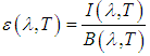 | (2) |
 is the radiance measured at the sensor for wavelength and temperature disregarding the effects of the atmosphere. Equation (2) is a ratio of the radiance of a given material and the radiance of a blackbody under the same temperature and wavelength. Then, for any real material, and knowing the emissivity and the target's temperature, from the Equation 2 the radiance measured at the sensor can be written as:
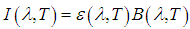 | (3) |
 | (4) |
 , and radiance measured by the sensor
  . This non-linearity contributes to multiply the effects of atmospheric scattering, emission effects in scenes with more complex geometries, scenes with heterogeneity of the atmosphere, and scenes with different adjacent surfaces (Collins et al., 1999 and 2001).Due to the presence of the atmosphere, the radiance reaching the sensor should, most of the time, be corrected for the emission effects, atmospheric scattering and attenuation, before the application of some of the methods discussed in this paper. In the literature, the radiation measured at the sensor including the atmosphere contribution is,
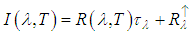 | (5) |
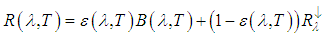 | (6) |
 is the down-welling spectral radiance that strikes the Earth's surface from scattering and from the atmospheric emissions,
  is the up-welling spectral radiance of the atmosphere that reaches the sensor,
  is the spectral transmissivity of the atmosphere and
  is the radiance measured in soil.In this work the main methods used by the scientific/academic community will be addressed, many of which served as the basis for newer and more complex methods. These methods are most applicable, because require less restrictions on the type of sensor, target, number of images and the number of spectral bands. There are other methods applied to more specific cases and will not be covered in this research.
 2. Problems to Separate Temperature / Emissivity
- The temperature and emissivity separation is complex due to the existing non-linear relation between the temperature and radiance (Li et al., 1999; Collins et al., 2001). The radiance can be calculated using the Planck’s function and target emissivity (for a given wavelength and temperature). Regardless of the number of spectral bands used for radiance measurements, there will always be one more variable than the measurements before. For example, a radiometer with N bands have N spectral radiance measurements and N + 1 variables (N emissivities for each band and a temperature T). This makes the system undefined, since it has more variables than equations, unless additional restrictions are included in the system.Another problem in the retrieval of terrestrial parameters is the interference from the atmosphere, especially in humid environments. Therefore, atmospheric corrections must be performed whenever possible. However, for such a correction, auxiliary data are required, and often are not available, so that the atmospheric correction becomes an additional problem especially if atmospheric models are used that are not consistent with the studied area.
3. Temperature and Emissivity Separation Methods
- Several temperature and emissivity separation methods have been developed in recent decades and many others are currently under study. All of them aim to separate temperature and emissivity information. However, there is a problem common to all methods, which is due to more variables than equations. Therefore, to mitigate this problem, each method is designed to be applied to specific conditions, and must satisfy a set of hypotheses, so that the result obtained is more reliable. With such restrictions, it is clear that the best result is directly related to the choice of the method that meets all the hypotheses and conditions, or the method that least violate them. These methods can be divided basically into three major groups (Gillespie1 1992): temperature enhancement and compositional data simultaneous (Spectral Ratio) temperature enhancement and individual compositional data (Two Temperatures Methods, Spectral Indexes of Independent Temperature, Re-normalization of Emissivity Method, Reference Band Method, Normalized Emissivity Method, Alpha Residues Method, Maximum-Minimum Difference Method, Grey Body Method) and hybrid highlights (Highlight Contrast by Decorrelation). Another important definition, which can be used to subdivide the methods, is related to those that calculate the relative emissivity and the ones that calculate the absolute emissivity. The term "emissivity on" is used when the emissivity value is calculated in relation to an emissivity of reference, and in this case, the result is the spectral curve of emissivity and not the value itself. The term "absolute emissivity" refers to the absolute value of this magnitude. The absolute emissivity is very important for surface temperature estimates (Sobrino and Jimenez-Munoz, 2002).
3.1. Contrast Enhancement by Decorrelation (CED)
- The contrast enhancement by decorrelation does not generate a quantitative result. The objective is to obtain a set of images from which one can form false-color compositions and extract visual information from the variations in temperature and emissivity.Different targets and differences in the composition of them account for differences in emissivity, even under isothermal conditions. However, this variation is not representative and makes the variability and emissivity contrast in the TIR be low, resulting in a high correlation for the different bands. One of the methods used to circumvent this problem is based on the transformation by Principal Component (PC) and is known as contrast enhancement by decorrelation (Soha and Schwartz 1978; Kahle and Rowan, 1980). Therefore, this method can easily be applied to images of any number of bands and can be summarized into four steps:1. Calculate the covariance matrix of the image and its eigenvalues;2. The image is transformed from the radiance domain into the PC's, and the transformed data have the property of being decorrelated;3. The most correlated PC's have their contrasts highlighted separately;4. The inverse transformation is applied, and the PC's return to space radiance.In general, the hues before and after transformation are very similar while the saturations are increased. In this sense, a false-color composition (RGB) of these images shows emissivity differences such as color variation and differences in temperature are shown as intensity variations.
3.2. Spectral Ratio (SR)
- The ratios between the radiances are less sensitive to small variations in temperature, unlike the radiances itself (Watson1 1992). Therefore, only an approximate value of temperature is necessary to determine the emissivity ratio with high precision.In this method, is proposed to use spectral ratios between adjacent bands because such ratios are efficient in detecting emissivity variations, however, have their limitations to the analysis of the entire spectrum. Initially, the presence of the atmosphere will be disregarded (Equation 3), thereby the radiance ratio is given by:
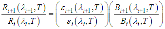 | (7) |
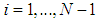 . Apparently, the problem of more variables than equations persists; however, the ratio
 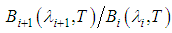 it is much less sensitive to small variations in the temperature that only the term
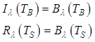
  (For the range of land temperatures and wavelengths between 8-14μm). There are several ways to estimate the temperature from the thermal radiance, however, an independent method of the prior knowledge of the geology of the area is to reverse Equation (3) to calculate the brightness temperature
  :
: | (8) |
 , as
, as  . Thus
 , where
  represents the best estimate of the surface temperature.Considering the atmosphere's contribution, given by Equations (5) and (6), we have three possible cases:CASE 1 - Neglecting
  the ratio in Equation (5) is:
 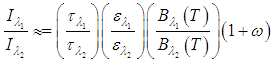 | (9) |
 , which is valid for daily data, since the atmosphere is partially transparent in this spectral region, follows that the 2nd term of the sum
  in Equation (9) can be neglected.CASE 2 – Including
  , and if there is a large enough area for calibration as a body of water, for example, the upward radiance can be estimated, and the measured radiance, corrected. A residual error of upward spectral radiance introduces a secondary term in the last parenthesis of the Equation (9) with the form
 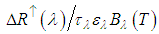 . For data acquired in suborbital, this error level is less than or equal to
  in Equation (9) and can be neglected.CASE 3 - With full atmospheric correction when the atmospheric parameters in Equation (6) can be estimated, the ratio of the corrected radiance, is given by:
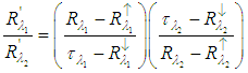 | (10) |
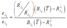 | (11) |
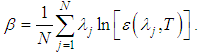
3.3. Spectral Index Independent of Temperature (TISI)
- This method was first proposed by Becker and Li (1990), and subsequently corrected by Becker and Li (1995) and Li et al. (1999). Using Equation (5) the band brightness temperature and the surface brightness temperature respectively are defined as:
 | (12) |
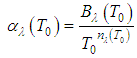
 , it was shown by Hardy et al. (1934) and Slater (1980) that the following approach for the Planck function is valid:
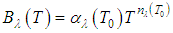 | (13) |
 and
and  are constants related to band
  and the temperature
  . The band constants
  and
and  are, respectively, given by:
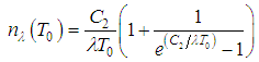
 Thus, from Equations (18), the band radiance
  can be estimated to an approximate temperature
  by:
by: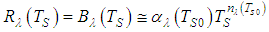 | (14) |
 . Now it is possible to rewrite Equation (12) as:
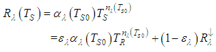 | (15) |
 is the kinetic temperature.If, for each radiance, the term
  can be neglected, Equation (15) becomes:
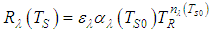 | (16.a) |
 | (16.b) |
 | (17.a) |
 | (17.b) |
 and
and  the equation
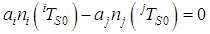 . Using
  and
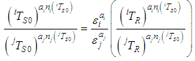
and  the temperature on the left side of the Equations (17.a) and (17.b) can be eliminated. Using these equations, it is easy to define an independent index of temperature:
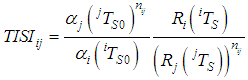 | (18.a) |
 | (18.b) |
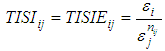 | (19) |
 on Equation (19):
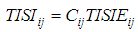 with:
with:  where
where 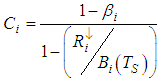 and
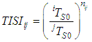
and 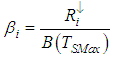 where
where  being the highest surface temperature of brightness found between the bands for a given pixel. This temperature of choice is the best approach for the kinetic temperature, allowing calculating efficiently the term
 .From this index
  it is possible to calculate the spectral emissivity, only if we know the upward atmospheric radiance in all bands, and the emissivity of a reference band (Becker and Li, 1990).
3.4. Reference Band Method (MBR)
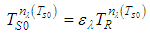
- Kahle et al. (1980) developed a method that assumes that a particular band (band r for example) has constant emissivity for all pixels. The selection of this band is subject to prior knowledge of the target in analysis and its emissivity. Knowing the atmospheric parameters
 of this band, it is possible to calculate an approximation of the surface temperature
  for each pixel given from the measured radiance
  using the inverse of Equations (5) and (6):
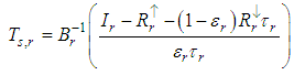 | (20) |
 | (21) |
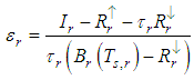
3.5. Method of Normalized Emissivity (MNE)
- Developed by Gillespie (1985) and more sophisticated than MBR (Gillespie et al. 1999) one assumes a single value for the maximum emissivity in each of the N bands, for all pixels of this band. Therefore, from the measured radiances, from an emissivity reference, and from Equation (10), are obtained N temperatures for each pixel. In each pixel, the highest of these temperatures is selected as the surface temperature of brightness. This temperature is used to calculate the new emissivity for all bands. The calculation of the remaining emissivities is performed as in MBR. The temperatures are calculated as:
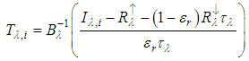 where
where  is the referece emissivity,
  is the radiance measured in band,
  for pixel
  , the terms
  ,
,  and
and  are, respectively, the upward radiance, the downward radiance and
  is the atmospheric transmissivity for band
  . Thus, the emissivity for pixel i is calculated by the equation,
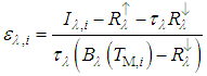 with
with  being the highest temperature of the calculated temperatures for pixel i.
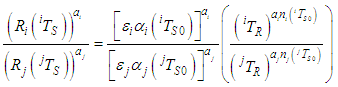
3.6. Method of the Alpha Residues (α-RM)
- The method was first proposed by Green and Craig (1985) under the name of Logarithmic Residues (LR), but has been modified by several authors and the final version developed by Hook et al. (1992). However, this method is still image dependent, in other words, dependent on information of the scene or analyzed region. However, it uses the approximation of Wien to Planck's function to isolate the temperature. The expression for the LR is given by:
 | (22) |
 and wavelenghts close to
  have maximum error of 1% (Siegel e Howell, 1982; Grondona et al., 2013). From the LR, arises the α-RM, which is an improved and simplified LR (Hook et al, 1992; Kealy and Hook, 1993; Gillespie et al, 1999), where the method's image-dependency is eliminated.Taking the average, over all bands of Equation (3) we have:
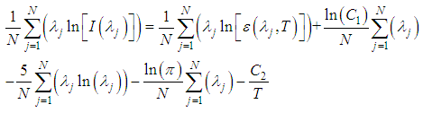 | (23) |
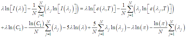 | (24) |
 | (25) |
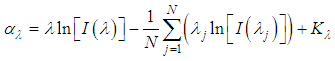 | (26) |
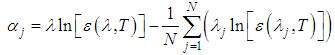
 is given by,
 | (27) |
 is the difference between the linearized equation of radiance and the radiance linearized average over all bands, for a particular pixel. Therefore, a set of temperature independent equations are obtained, and can be calculated using Equation (26) from the scene data. It should be noted that the alpha residues retain the shape of the emissivity spectrum but not its absolute value, and, for the purpose of laboratory data comparison (Equation (25)) with field data (Equation (26)), conversion of the former data should be performed. Using emissivity data obtained in laboratory, upon application in Equation (25) it is possible to calculate
  , and then compare it with the scene data from Equation (26). However, to extract the emissivity of the scene directly from Equation (25), it is necessary to solve
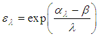 | (28) |
 However, the calculation of the emissivity in Equation (28) is not possible because
  is not known. One way to calculate the variable
  is considering the spectral behavior in the thermal infrared of common targets. Thus, from the variance of a set of various soil types, igneous rocks and sedimentary rocks, Equation (28) can be solved. To estimate the term
 , a regression is used. Given by:
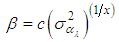 | (29) |
3.7. Maximum-Minimum Method Difference (MMD)
- Proposed by Matsunaga (1994) and using the relation between the average emissivity
 and the difference between maximum and minimum variation. Based on the average spectrum emissivity and using an iterative process, the mean emissivity is corrected by estimate according to the difference between the maximum value and minimum emissivity of the previous iteration. At the end of the process, the temperature is finally calculated. This process can be described in five steps (Matsunaga, 1994; Gillespie et al, 1999; Coll et al., 2007.):1. Initial estimate of emissivity spectra, usually with MNE.2. The MMD is calculated from the previous step for the first iteration, in the remaining, MMD is calculated from adjusted emissivity spectra as,
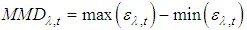 | (30) |
 and
and  are, respectively, the maximum and minimum emissivities for the band
  , at iteration
  .3. The new average emissivity,
  , is calculated using the expression
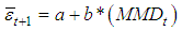 | (31) |
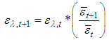 | (32) |
 and its respective radiance.The iterative process continues from step 2 to step 5 until the temperature difference between iterations is less than a predetermined number
  , so that
 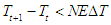 .
.3.8. Gray Body Method (MCC)
- Proposed by Barducci and Pippi (1996) MCC is based on the assumption that the emissivity spectrum of the target concerned is flat enough so that the variation of the emissivity is negligible, in other words, the emissivity varies little in relation to wavelength. This hypothesis is often observed, particularly in emissivity spectra obtained in laboratory, or from hyperspectral thermal sensors, and can be written mathematically as:
 | (33) |
 | (34) |
 being the average emissivity for band
  .The hypotheses of the Equations (33) and (34) are conceptually the same, but each one applies in a given situation. While the first serves for applications with a continuous spectrum, the second applies to spectrum intervals, in other words, the hypothesis of Equation (33) is wider than the case of Equation (34).Rewriting the radiance, as
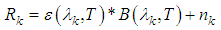 | (35) |
 it is an additive term with zero mean due to noise. Then the algorithm for estimates for the temperature
  and emissivity
  that minimizes the error
  is given by,
 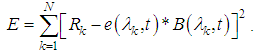 | (36) |
 represents the real values of emissivity and temperature, while e and t are, respectively, the estimates of these variables. Expressing the terms e and t by:
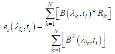 | (37) |
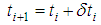 | (38) |
 | (39) |
 , and, from this temperature, the first estimate for the emissivity
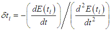
  is calculated. Then, the new temperature to be used in the next iteration is calculated, and a revised estimate is made for the emissivity, and so on. The process iterates until the calculated temperature minimize the Equation (36), in other words:
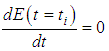 | (40) |
4. Results and Discussions
- Each of the nine methods analyzed have mathematical properties and applications that are directly related to the quality and accuracy of the final result. It is very important to understand these limitations for a suitable choice of the method to be used.The RCD produces a false-color composition which shows variations in emissivity/temperature and variations in color/intensity respectively, but does not return numerical values for the temperature/emissivity. The method is image-dependent, in other words, the result of using the entire scene is different from the result obtained using only a cut-out of the original scene. When there are large variations in temperature within the image, data may be degraded, since cold areas will be darker in color, masking minor variations (emissivity). The method applies to multiple targets simultaneously, and atmospheric correction is needed once the emissions from the atmospheric scattering attenuates the soil response.The RE has little sensitivity to small changes in temperature, and since the bands are close enough, one might consider emissivity equal between these bands. When that happens, the ratio between these radiances produces an error smaller than 1%. The method is applicable to multiple targets simultaneously, but direct comparison of radiance cures/emissivity with the ratio curves is not possible. For such a comparison, one should convert the radiance/emissivity curves into ratio curves or the opposite (using an emissivity of reference, thereby obtaining the relative emissivity). In this method, the atmospheric correction is necessary because the ratio enhances the picture noise, both the intrinsic obtained from the scene as the noise arising from atmospheric scattering. This method is applicable to any sensor with at least two bands.The MDT has a single hypothesis, in which the emissivity is invariant in time, this allows for directly calculate the emissivity data. This method combined with the RS is very effective in mineral exploration, however, their hypothesis, can be applied to multiple targets simultaneously. The best results are obtained for data with low emissivity and/or small variation in temperature/emissivity from the observations. However, the method is not yet well established for vegetation, and is definitely invalid for transient changes (eg mixing of soils, variations in surface materials, rainfall or other events between observations). Other possible sources of error are: registration of images, the enhancement of noise in the existent ratio (that is why the atmospheric correction is very important). Direct comparison of data is not possible and the recovered emissivity is relative.The TISI is practically independent of temperature, the ratios TISI and TISIE are close, and, as the temperature increases, this difference decreases. The difference between these levels is approximately 1%, and can be even smaller with higher emissivity and better atmospheric conditions. The TISI is directly calculated from the radiance data, and is very sensitive to variations of the surface features. As Becker and Li (1990), this index can be up to 12 times more accurate than a simple spectral ratio. However, due to the existing ratios in the method the lack of atmospheric correction (or non-adequate correction) significantly increases the noise in the data. For the calculation of emissivity, an emissivity reference is required. The method is applicable to sensors with at least two bands, and is readily applicable to more than two bands simultaneously. In addition, most suitable indexes to an application may exist, depending on the combination of used bands (Becker and Li, 1990). Finally, the index is not very sensitive to the characteristics of vegetation unlike exposed soils.The MBR had great importance in research with TIR, and is also called, for this reason, a model emissivity method (Gillespie et al., 1999). For the application of this method it is necessary a priori knowledge of the target, the maximum value for the emissivity and the band can be selected. For silicates, this band is always located at longer wavelengths of the TIR and maximum emissivity is ≈ 0.95. The problem with this method is to assume that all image pixels in a given spectral band, have the same emissivity. Targets such as vegetation, snow and water temperature would be underestimated, as its emissivity is higher than previously proposed. So, this method does not produce good results, simultaneously, for targets with very different emissivities. The method allows the direct comparison of data because it returns the absolute emissivity and can be applied to sensors with one band or more. Because of the simplicity of the method, the contribution from the atmospheric scattering suffers no enhancement, but depending on the study and the desired accuracy, the atmospheric correction is essential.The MNE inherits all RCM features and is less prone to errors. In this method, the maximum emissivity occurs in the band that has the maximum temperature (for that pixel). The accuracy of the MNE depends on the initial value of the maximum emissivity used, however, it is unable to produce good results, simultaneously for targets with very different emissivity. If a target with emissivity higher than the emissivity maximum initially set, the temperature for this target will be underestimated. The recovered emissivity is absolute and is also applicable to sensors with single or multiple band, and the atmospheric correction has the same treatment as in RCM.In α-RM, the comparison of data (laboratory-field) is not direct, thuss conversion is required for the form of alpha residues (laboratory data), or alpha residues to relative emissivity according to Equation (26). The main advantage of this method is its independence from temperature, with low noise propagation from one band to others. Also, results are generated for different targets simultaneously preserving the spectral emissivity curve, but not its amplitudes. The method is image-independent, then, working with the full scene, or only part of it, does not insert errors. A disadvantage is the use of an approach to the Planck function (Wien's approach), but since the restrictions are observed, errors are less than 1% (Grondona et al., 2013). Finally, even with little noise propagation, the atmospheric correction is needed to minimize the error in the method.In the MMD, the temperature is relatively insensitive to multiple scattering of radiation and thermal radiance downward, inside an element of the scene, but the (relative) calculated emissivity is more sensitive to these factors. The accuracy of the MMD and the MEN are similar, but the first depends on the accuracy of the relation between and NEΔT. The MMD mean square error is smaller than the MEN, except NEΔT> 0.3K. In general, the MMD ends up being more accurate and more sensitive to measurement errors, that NMS. For greater reliability in the result of the MMD, the atmospheric correction is required, and even applicable to multiple targets simultaneously. Preferably, one should apply the method to targets with little variation in emissivity. The method requires at least one band for its application.MCC is able to get the temperature and emissivity of a target with no a priori knowledge about the target, by simply an initial approximation for the temperature. For hyperspectral sensors, the algorithm is promising, since the possibility given by Equation (45) occurs more easily. However, for most targets of terrestrial coverage, this assumption is not fulfilled, particularly in multi-spectral sensors due to their "small" number of bands in the thermal region and its distribution, respectively (Gillespie et al., 1999). The method is sensitive to measurement error, especially when using the assumption of Equation (46), as well as errors resulting from atmospheric scattering. For this reason, the atmospheric correction is required. The MCC calculates the absolute emissivity and allows direct comparison of the data. Due to the construction (hypotheses) method, it requires at least two bands for application.Note, that a common source of errors to all methods to be taken into account are areas with clouds. Despite the TIR wavelengths are less susceptible to interference caused by clouds than the regions of visible and near infrared wavelengths, this target is not invisible in TIR, and the analyzed methods do not apply in such areas. Clouds are water vapor, which in turn is a major cause for problems in interpreting TIR, and application of cloud filtering methods degrades the data since it has no real value of reflectance/radiance of the targets below the clouds, but only an estimate of it. It should also be considered that the spatial resolution can be a problem, but this problem is mainly related to the studied scale, and has little to do with the method chosen.
5. Conclusions
- All the methods described above represent the largest and main part of the existing methods of temperature and emissivity separation developed in the last four decades. Other more recent methods are offered, but are applied in more specific cases of sensors, targets or certain studies, and they are not part of the objective of this work. The methods covered in this work, although they are applicable in various situations, produce more accurate data if applied according to its restrictions / limitations. All these methods have been developed based on laboratory data, so it should be noted that all require the atmospheric correction data. Some are more sensitive to errors of this influence (if not performed correctly), others are more robust, but the best results will be obtained with the atmospheric correction using location data to study the same day of a worked scene. The most sensitive methods are those that (at some point) have a ratio of spectral bands, or some kind of algebraic manipulation that can supress noise, among these methods are RE, MDT, TISI and α-RM.Another important point is that most methods have been developed for the study of soils and rocks, once the TIR is intended for this type of study (mainly sensor technological limitations). The vegetation has little differentiation in this region of the electromagnetic spectrum, nevertheless, some of these methods may return information for vegetation studies.In general, MEN is what produces the best results when one has priori knowledge of the maximum target emissivity for any type of study. The TISI and α-RM give good estimates for the relative emissivity of targets (vegetation and soil) from a reference emissivity without the knowledge of the temperature, and the α-RM is easier to implement when compared to TISI. The MCC is the most suitable for hyperspectral sensors and targets that have little variation in emissivity for two adjacent bands.These methods meet in a satisfactory manner a wide range of applications, however, due to technological advances in the sensors and the need for studies and more accurate monitoring of the Earth's surface, research is necessary for more accurate / precise methods that are less susceptible to errors in separation of the temperature and emissivity of targets.
ACKNOWLEDGEMENTS
- The authors would like to thank the Geological Remote Sensing Laboratory (Laboratório de Sensoriamento Remoto Geológico - LabSRGeo) of Federal University os Rio Grande do Sul – UFRGS, and FAPERGS – Project-2275-2551/14-1.