-
Paper Information
- Next Paper
- Previous Paper
- Paper Submission
-
Journal Information
- About This Journal
- Editorial Board
- Current Issue
- Archive
- Author Guidelines
- Contact Us
American Journal of Environmental Engineering
p-ISSN: 2166-4633 e-ISSN: 2166-465X
2016; 6(4A): 116-118
doi:10.5923/s.ajee.201601.17

Comparing Meandering Parameters from the Distinct Autocorrelation Functions
 Abstract
 Reference
 Full-Text PDF
 Full-text HTML
Luís G. N. Martins1, Michel B. Stefanello1, Gervásio A. Degrazia1, Lidiane Buligon2, Luca Mortarini3, Lilian P. Moor1, Debora R. Roberti1, Felipe D. Costa4, Franciano S. Puhales1, Domenico Anfossi3
1Departamento de Física, Universidade Federal de Santa Maria, Santa Maria, Brasil
2Departamento de Matemática, Universidade Federal de Santa Maria, Santa Maria, Brasil
3Institute of Atmospheric Sciences and Climate (CNR/ISAC), Unit of Turin, Turin, Italy
4Programa de Pós-Graduação em Engenharia, Universidade Federal do Pampa, Campus Alegrete, Alegrete, Brasil
Correspondence to: Gervásio A. Degrazia, Departamento de Física, Universidade Federal de Santa Maria, Santa Maria, Brasil.
| Email: |  |
Copyright © 2016 Scientific & Academic Publishing. All Rights Reserved.
This work is licensed under the Creative Commons Attribution International License (CC BY).
http://creativecommons.org/licenses/by/4.0/

The following study employs two different autocorrelation functions (ACF) to obtain the principal parameters that describe the behavior of the low-wind meandering phenomenon. The looping parameter (m) and the meandering time scale (T*) were estimated from the fit of 828 experimental ACF evaluated from measurements accomplished at the Santa Maria micrometeorological site (Santa Maria, south of Brazil). The results show that both meandering ACFs appropriately fit the negative lobes and the oscillatory behavior observed in experimental meandering ACFs. The T* parameter, obtained from the distinct ACF formulations, agrees in most of the analyzed cases. However, substantial differences between the values of the m parameter, obtained by the two formulations, are observed. This difference is more evident for higher values of m. This highlights the distinct functional form that describes the turbulence in the meandering ACF.
Keywords: Wind meandering, Autocorrelation functions, Low wind
Cite this paper: Luís G. N. Martins, Michel B. Stefanello, Gervásio A. Degrazia, Lidiane Buligon, Luca Mortarini, Lilian P. Moor, Debora R. Roberti, Felipe D. Costa, Franciano S. Puhales, Domenico Anfossi, Comparing Meandering Parameters from the Distinct Autocorrelation Functions, American Journal of Environmental Engineering, Vol. 6 No. 4A, 2016, pp. 116-118. doi: 10.5923/s.ajee.201601.17.
1. Introduction
- The velocity autocorrelation functions are important statistical quantities to describe atmospheric movements. Such functions can be used to calculate the dispersion parameters associated to the turbulent diffusion modeling studies in the planetary boundary layer (PBL). Based on the Taylor Statistical Diffusion Theory, the following formula has been proposed by Frenkiel [1] and [2] to represent the autocorrelation functions describing the connected states between turbulent and non-turbulent (submeso motions e.g. [3]) movements.
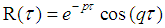 | (1) |
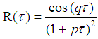 | (2) |
 , the Lagrangian integral time scale for a fully developed turbulence, and m the loop parameter, which controls the meandering oscillation frequency associated to the horizontal wind. The m parameter controls the negative lobe absolute value in the autocorrelation functions and as a consequence defines the meandering phenomenon intensity [6]. Following [2] and [7] p and q are defined by the relations:
 | (3) |
 | (4) |
 (u and v are the horizontal and lateral turbulent velocity components and T is the temperature), are calculated. Furthermore, the looping parameters and the meandering periods derived from Eq. (1) are compared with those obtained from Eq. (2).
 2. Results and Discussion
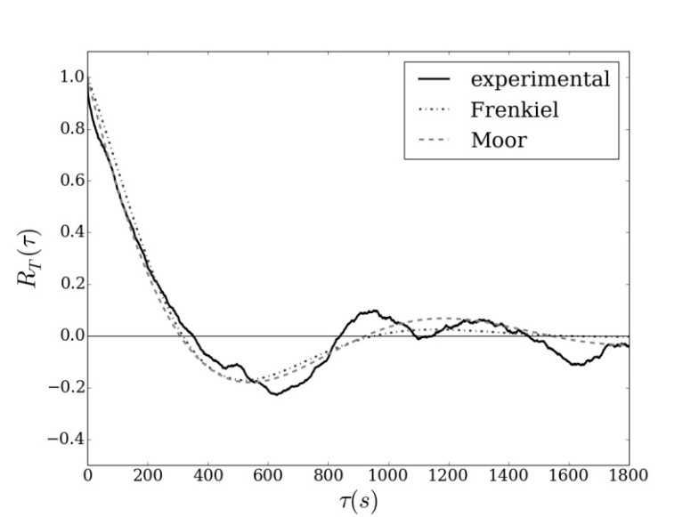
- In this section, we analyze low-wind speed data to evaluate experimental autocorrelation functions. These experimental curves, presenting negative lobes, are fitted by mathematical formulations provided by the Eqs. (1) and (2). Therefore, Eqs. (1) and (2) are mathematical representations that reproduce the observed meandering curves and are used to obtain the loop parameters and the meandering periods. The low-wind speed dataset employed in this analysis were measured in a micrometeorological station (UFSM, Rio Grande do Sul, Brazil) between November 2013 and December 2014. Observations of wind speed and temperature were sampled by a sonic anemometer installed at 3 m in a tower at a frequency of 10Hz. Figures 1-3 show peculiar patterns of the comparison among the velocity and temperature ACFs calculated on the Santa Maria low wind speed dataset (continuous line) and the associated best fits (dotted and dashed lines) calculated from the ACFs (Eqs. (1) and (2) respectively).
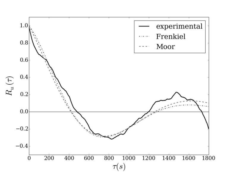 | Figure 1. Comparison between the ACF estimated on the Santa Maria dataset (continuous line) and the associated best fits (dotted and dashed lines) for the u component, evaluated from Eq.(1) and from Eq. (2) on April 25 of 2014, 00:00LT;  |
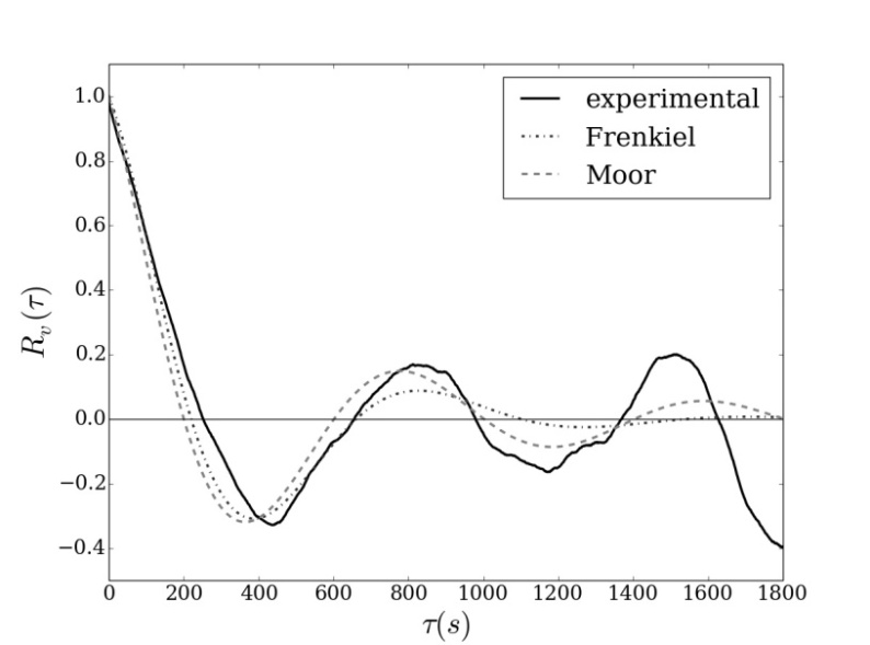 | Figure 2. As in Fig. 1, for the v component |
 | Figure 3. As in Fig. 1, for the temperature |
 . Eq. (4) provides the meandering characteristic time scale (meandering period). From this equation values of the magnitude of T* were obtained. Figure 4 shows the scatter plots of T* calculated from Eq. (1) (x-axis) and Eq. (2) (y-axis). It can be seen that there is a very good agreement between the magnitudes of T* obtained from the two mathematical formulations. This behavior is evidenced by the fact that most of the T* values are situated on the line of perfect agreement. From Eq. (5) the loop parameter m can be estimated. Figure 5 exhibits the scatter plot of the m values obtained from Eq. (1) (x-axis) and Eq. (2) (y-axis). Looking at this scatter plot, it is evident that the loop parameter estimated from Eq. (2) presents greater magnitudes than the one provided by Eq. (1). Furthermore, it is important to note that the Figure 4 present a linear relation between the m values calculated from Eqs. (1) and (2).
 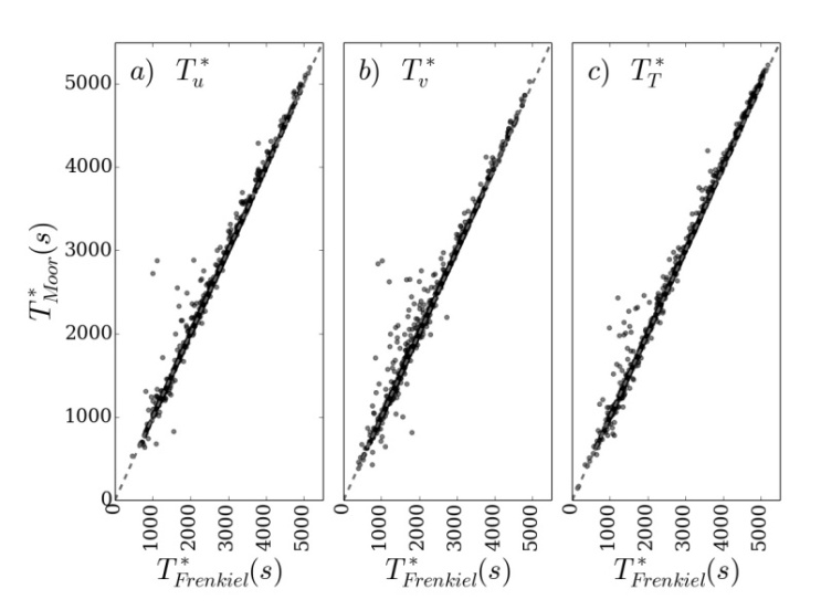 | Figure 4. Meandering period for all low wind dataset |
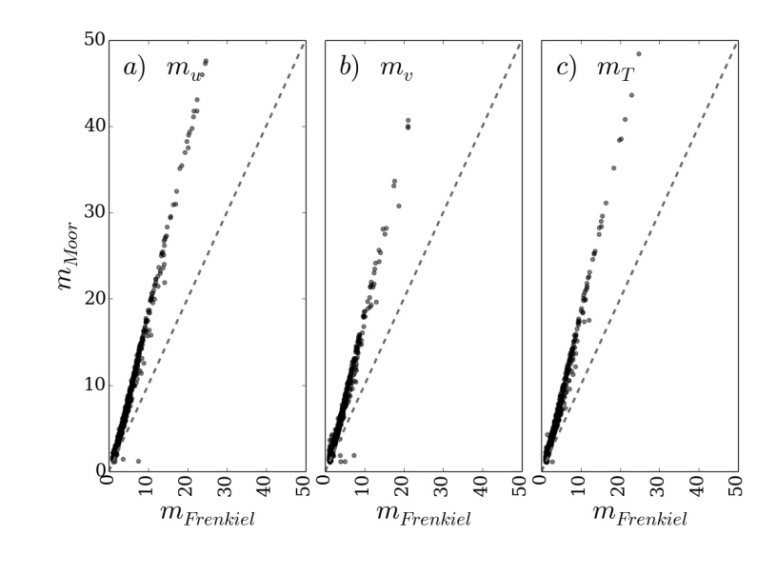 | Figure 5. Loop parameter (m) for all low wind dataset |
3. Conclusions
- We present a comparison between two mathematical formulations that describe the negative lobes associated to the observed meandering ACF. The analysis shows that both mathematical expressions appropriately fit the experimental data. The oscillatory behavior presents in the meandering motion are equally well described by both representations. Thus, the meandering time scale can be estimated independently of the ACF formulation chosen. On the other hand, the m parameter is larger for the case in which the turbulence movement is represented by the binomial function. This last decreases more slowly than the exponential function.
ACKNOWLEDGEMENTS
- The authors would like to thank the CNPq and Capes for partial financial support of this work.