Adrián R. Wittwer1, Rodrigo Dorado2, Gisela Alvarez y Alvarez1, Gervásio A. Degrazia3, Acir M. Loredo-Souza2, Bardo Bodmann2
1Facultad de Ingeniería, Universidad Nacional del Nordeste, Resistencia, Argentina
2Universidade Federal de Rio Grande do Sul, Porto Alegre, Brazil
3Universidade Federal de Santa Maria, Santa Maria, Brazil
Correspondence to: Adrián R. Wittwer, Facultad de Ingeniería, Universidad Nacional del Nordeste, Resistencia, Argentina.
| Email: |  |
Copyright © 2016 Scientific & Academic Publishing. All Rights Reserved.
This work is licensed under the Creative Commons Attribution International License (CC BY).
http://creativecommons.org/licenses/by/4.0/

Abstract
The interaction between the incident wind and wind turbines in a wind farm causes mean velocity deficit and increased levels of turbulence in the wake. The turbulent flow is characterized by the superposition of wind turbine wakes. In this work, the technique of turbulence spectral evaluation for reduced scale models in a boundary layer wind tunnel is presented, and different measurements of velocity fluctuations are analysed. The results allow evaluating the spectrum for different frequency ranges and the differences of the spectral behaviour between the incident wind and the turbine wake flow.
Keywords:
Wind turbine, Turbulent wake, Reduced scale models
Cite this paper: Adrián R. Wittwer, Rodrigo Dorado, Gisela Alvarez y Alvarez, Gervásio A. Degrazia, Acir M. Loredo-Souza, Bardo Bodmann, Flow in the Wake of Wind Turbines: Turbulence Spectral Analysis by Wind Tunnel Tests, American Journal of Environmental Engineering, Vol. 6 No. 4A, 2016, pp. 109-115. doi: 10.5923/s.ajee.201601.16.
1. Introduction
Different aspects, such as the deficit speed in the case of successive generators and turbulence levels in the wake of wind turbines, need to be considered in the analysis of fluid-structure interaction between the incident wind and the turbine in a wind farm. In a wind turbine farm, the turbulent flow is characterized by the coexistence and superposition of multiple wakes and wind potential losses due to the wake effects that can reach up to 20% of the total energy. Some studies show that wind turbines operating in a farm may have a drop in generated power up to 40% compared with the case of an independent turbine [1] [2]. Other investigations analyse the power degradation produced from the second row of wind turbines and its evolution [3].The fatigue problems in the turbines are associated with the turbulence intensity that also have a direct impact on forces and moments in wind turbine blades. Although there are experimental and computational research papers that improve the understanding of these problems, there are no sufficiently reliable models to predict the spatial distribution of turbulence in wind farms.The difficulties involving the coexistence of multiple overlapping wakes, the boundary layer effect, the local topography, the turbulence levels and thermal stratification suggest the complementary use of different types of approaches to characterize the turbulent flow in wind farms. Wind tunnel experimentation using reduced scale models allows to reproduce the interaction phenomena under controlled conditions. There are studies focused on boundary layer physical simulation [4] in the wake structure of a wind turbine [5] and others evaluate the effective turbulence of a wind farm [6] [7] [8]. In general, this type of study determined that basic analysis models overestimate wind farms efficiency, and calculate wakes shorter than real ones.This work is a first of a series of experimental studies of the spectral characteristics of turbulence in the wake of a wind turbine. Longitudinal velocity fluctuations were measured in the incident flow and in the wake of a wind turbine reduced model in a wind tunnel test section. In these experiments, the adequacy of spectral technique and changes in the turbulence spectral composition of the incident wind and the wake are analysed.
2. Flow Characteristic Parameters in Aerogenerators
When wind approaches the wind turbine rotor there is a reduction of the axial velocity component before that air passes the rotor plane. This reduction is the deficit of axial velocity component and defines the axial induction factor:  | (1) |
where U∞ is the free-stream velocity and U1 is the velocity in the rotor plane. After crossing the rotor plane, the axial velocity component decreases and considering a simplified dimensional analysis, becomes U∞ (1-2a) far downwind. When the flow passes through the rotor, a pressure drop occurs. The decrease of flow velocity after passing through the rotor undergoes pressure recovery, until the atmospheric pressure is restored. In this idealization, it is considered that half of the induction occurs before the rotor and the second half of the induction occurs behind. Another factor used to describe velocity field around a generator is the tangential induction factor a’, product of the flow rotation in the wake.  | (2) |
where Ω is the angular velocity of the rotor and ω the rotational velocity in the wake. Higher values indicate that the power produced will be low and there is a large amount of kinetic energy associated with the wake rotation.The axial induction factor a is directly related to the power extracted by the turbine. If the incident wind stops completely due to turbine blade action (a = 1), there would be no power extraction because flow is not passing through the rotor plane. On the other hand, if there is no change in wind speed exceeding blades (a = 0) there would not be power extraction, and the kinetic energy remains constant before and after the rotor. The power extracted by the turbine is defined by: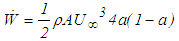 | (3) |
where ρ is the air density and A the rotor area. The power of the incident wind is: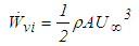 | (4) |
The coefficient of power Cp is the fraction of incident wind power extracted by the rotor  and is a measurement of how efficiently the wind turbine converts the energy in the wind into mechanical energy.Finally, there is another important parameter in the analysis of the operational characteristics of a wind turbine called tip speed ratio (λ). It is the ratio between the tangential speed of the tip of a blade and the free stream velocity:
 | (5) |
where r is the radius of the rotor. The graph of power coefficient Cp as a function of the tip speed ratio λ is a characteristic curve of this type of turbine.
3. Instrumentation and Experimental Technique
The experiments were developed in the wind tunnel “Jacek P. Gorecki” of UNNE, Argentina [9]. Figure 1 shows the atmospheric boundary layer (ABL) simulation devices and the turbine model in the test section of the wind tunnel. All longitudinal velocity fluctuation measurements were realized employing neutral ABL simulation obtained by the Counihan method (barrier, vortex generators and surface roughness). The simulated incident wind corresponds to a power law profile with an exponent α = 0.27 and a gradient height zg = 1.20 m. Wind tunnel measurements were made using a hot-wire anemometer connected to a data acquisition system (Figure 2). The wind turbine model corresponds to a three bladed UNIPOWER wind turbine, with a tower height of 100 m and a rotor diameter of 100 m (Figure 3). The scale of the model is approximately 1/450 and the model height is 0.33 m. Figure 4 shows the wind incident making rotate the turbine model.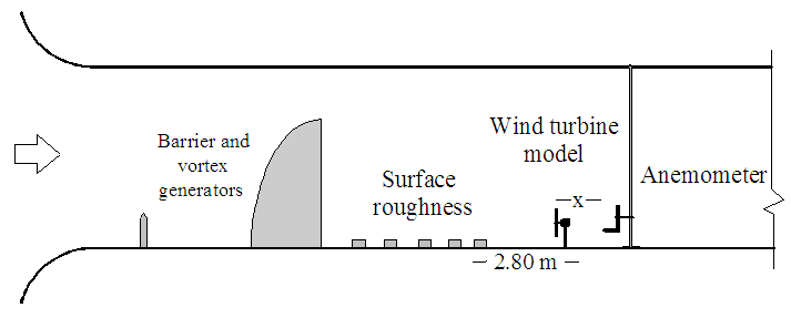 | Figure 1. ABL simulation devices and turbine model in the wind tunnel |
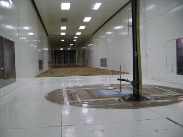 | Figure 2. Wind turbine model and measurement device in the test section |
 | Figure 3. Wind turbine model details |
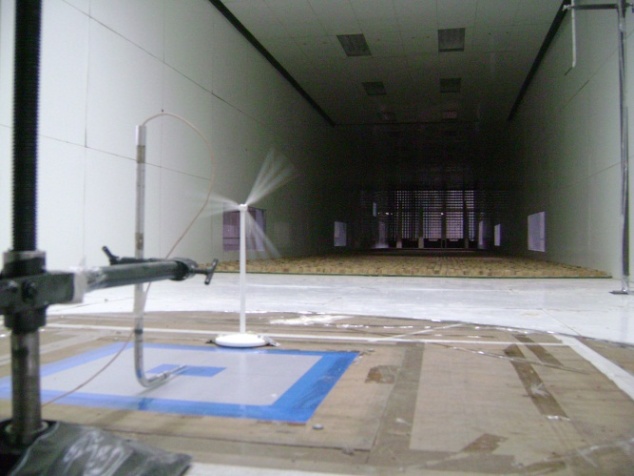 | Figure 4. Wind turbine spinning during test |
Measurements of velocity were performed at three different heights z, first with incident wind, and later, in the wake of the wind turbine model, at a distance of 2.8 m downwind of the model. Representative numerical series of velocity were obtained by a sampling frequency of 1024 Hz during 128 seconds. Before sample acquisition, an electronic low-pass filter was adjusted to 100 and 300 Hz.The Reynolds number | (6) |
is defined by the mean velocity U and the generator diameter ϕg and the test value of Re is 1.63 × 10⁵, being μ the kinematic viscosity of air. The rotational velocity of the wind turbine was estimated by image analysis and remained nearly constant during measurements, but it is important to note that it cannot achieve the values of the dimensionless speed ratio λ to ensure the similarity of phenomenon in the range of the proper operation of the generator.
4. Results
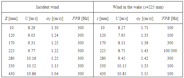
In this section the results obtained in the tests described in the previous section are presented. The main characteristics of the measuring points (height z, mean velocity U, standard deviation of velocity fluctuations σu) are indicated in Table 1. Frequency setting of lowpass filter (FPB) is also indicated. First, the mean velocity and turbulence intensity profiles are shown, and then the spectra corresponding to the longitudinal velocity fluctuation. The profiles were obtained considering 15 measuring points distributed between z = 10 mm and z = 640 mm, whereas for spectral analysis are considered only 7 points with incident wind and 7 points in the case of wind in the wake at x = 225 mm position (Table 1).Table 1. Main characteristics parameters
 |
| |
|
4.1. Mean Velocity and Turbulence Intensity Vertical Profiles
In Figures 5 and 6 vertical profiles of dimensionless mean longitudinal velocity U/Uref and the normalized turbulence intensity urms/Uref to the incident wind and in the wake generated by the wind turbine are indicated. Profiles measured at two locations (x = 225 mm and 1185 mm) downwind of the plane determined by the rotor blades are included, and the corresponding wind incident profile whose characteristics are close to the power law profile with exponent 0.19. The reference height is zref = 540 mm and was defined arbitrarily, so that the velocity variations which occur in the wake must be considered in relation to this reference. Mean velocity profiles indicate higher mean velocity decreases in the lower half region of the rotor and, as could be expected, in the downwind position closest to the model (x = 225 mm). For the other position (x = 1185 mm) one observes the trend towards reconstruction of the original profile. In the vertical distribution of the turbulence intensity, for the incident wind approximately constant values are checked at the bottom of the simulated boundary layer, up to z ≈ 300 mm, which is consistent with experimental values for boundary layer flow of this kind. The most visible increments of Urms/Uref are verified for the profile where the position is closest to the model (x = 225 mm), specifically in the measurement points located at the bottom and on the rotor shaft. In the far most downwind location (x = 1185 mm) approximately constant values are observed, indicating a vertical diffusion of the fluctuations which occur in the vicinity of the model. As in the velocity profiles, turbulence intensity was normalized with the mean velocity at a height zref = 540 mm, a parameter that must be considered when analyzing the change in the fluctuating values between profiles.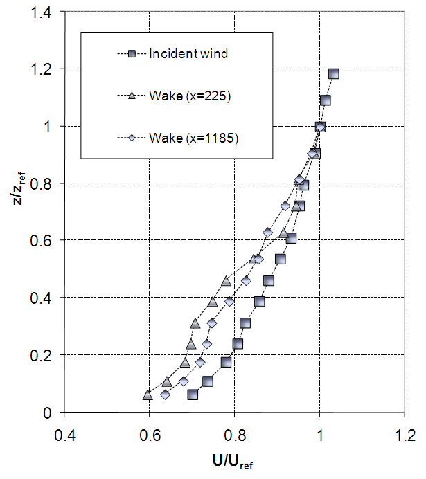 | Figure 5. Vertical profiles of dimensionless mean longitudinal velocity |
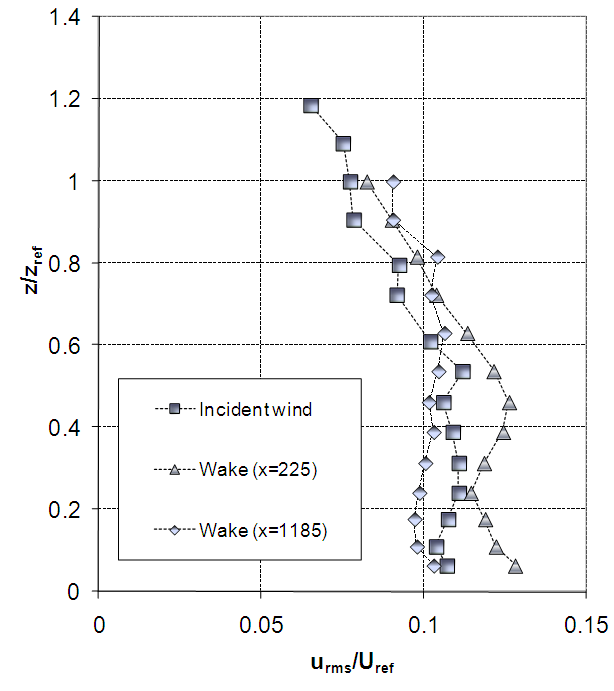 | Figure 6. Normalized turbulence intensity |
4.2. Evaluation of the Resolution on the Turbulence Energy Spectra
The auto-spectral density function or power spectrum represents the variation in function of frequency, of the mean square value of the velocity fluctuation as a function of time u(t) provided by a continuous number series acquired with a time interval t, and it is expressed by: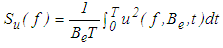 | (7) |
where Be is the bandwidth (spectrum resolution), and T is a suitable integration time depending on the scales of turbulence. The integral of this function allows obtaining the variance of velocity fluctuations σu2. To analyse the spectra in terms of its resolution based on the frequency, spectra in function of the number of blocks, number of values per block and averaging effect in one position (z = 170 mm) are evaluated. In Figure 7, based on the same measurement three spectra were obtained in this position for the incident wind. The spectrum identified as "z = 170 mm - low" describes the low frequencies, was obtained using 8 blocks of 16384 values and has less averaging effect. The second one, "z = 170 mm - medium" obtained from 32 blocks of 4096 values, allows to describe the intermediate and high frequencies. Finally, using 256 blocks of 512 values, the spectrum "z = 170 mm - high", describes of the high frequencies. In Figure 8, similarly spectra corresponding to the same vertical position (z = 170 mm) were obtained for the case of wind in the wake (x = 225 mm) which are descriptive of low, intermediate and high frequencies.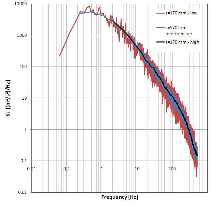 | Figure 7. Spectrum of incident wind obtained at z = 170 mm |
 | Figure 8. Spectrum of wind in the wake obtained at z = 170 mm and x = 225 mm |
This assessment is done to get a general impression of the spectral behaviour throughout the frequency range. Increasing the number of blocks, decreases the resolution at low frequencies, but the average of the blocks allows a better visualization of what happens in intermediate and high frequencies. In particular, for the measurements performed in this work, the composition of the spectra at low frequencies for the wind in the wake show no significant alterations and, therefore, the comparative analysis will be performed only by the descriptive spectra of the medium and high frequencies.
4.3. Evaluation of Spectral Configuration and Filtering Effect
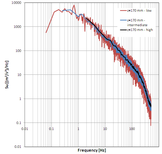
In Figure 9 spectra for incident wind in 5 different vertical positions are shown, indicating complementarily the -5/3 slope that defines the inertial region. In all cases the spectral resolution is defined by a series of 131072 values divided into 32 blocks of 4096. The analog signal is filtered by a low-pass filter at 300 Hz. A significant similarity between the spectra corresponding to z = 120, 225, 330 and 430 mm positions can be observed. The small differences that occur in the remaining spectrum (z = 10 mm) are most likely due to the proximity to the floor that generates boundary effects. | Figure 9. Spectrum of incident wind obtained in different positions with analog filtering at 300 Hz |
Similarly, in Figure 10 spectra for the wind in the wake (x = 225 mm) in the same vertical positions are presented, also indicating the slope -5/3. The spectral resolution is defined in the same way, but in this case the analog signal is filtered at 100 Hz. In this case, it is possible to verify more differences between the spectra, and even for intermediate and high frequencies different behaviours in lower positions at z = 225 mm and in the top two positions are visible. The effects of the analog filtering of the anemometer signal at different frequencies, in each situation can clearly be perceived. Also, the effects of the wind turbine model generate changes in the spectral configuration according to the analysed vertical position. To evaluate these effects, a comparative analysis of the spectra of incident wind and those obtained in the wake of the model is performed.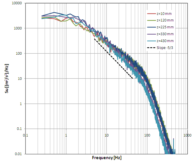 | Figure 10. Spectrum of wind in the wake obtained in different positions with analog filtering of 100 Hz |
4.4. Comparison of the Spectral Characteristics of the Incident Wind and the Wake of the Turbine
Finally, a comparison of the spectra obtained for the incident and in the wake of the wind turbine is performed. For a better visualization of the differences, in this analysis spectral resolution is used, employing 256 blocks to improve the effect of averaging. In Figure 11, spectra corresponding to the position z = 17 mm show some differences in the lower frequencies, and from 15 Hz, the separation of the spectrum in the wake relative to the clear definition of the inertial region (slope -5/3) in the spectrum of the incident wind. The effect is predictable from the additional turbulence produced by the turbine. Between 200 and 300 Hz, the effect of the low-pass filter is clearly perceived. In Figure 12, the spectral comparison in the position z = 225 mm (turbine shaft height) indicates a behavior very similar to the previous; only in the lower frequencies no differences are verified. Finally, in the z = 280 mm position, the separation of spectra is lower than in the two previous positions (Figure 13).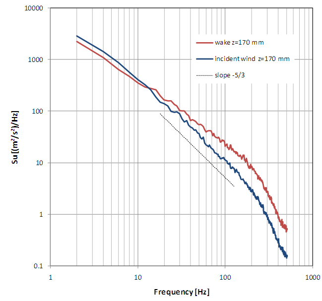 | Figure 11. Spectral comparison of the incident wind and wind in the wake for z = 170 mm |
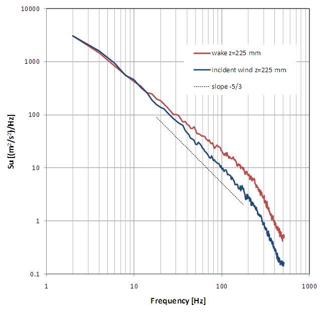 | Figure 12. Spectral comparison of the incident wind and wind in the wake for z = 225 mm |
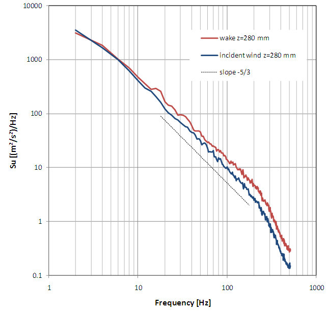 | Figure 13. Spectral comparison of the incident wind and wind in the wake for z = 280 mm |
In all positions an increase of fluctuation intensity in the wake with respect to incident wind was observed, however at z = 280 mm position, the increase is higher (around 6%). The bi-logarithmic representation of the spectra cannot display this behaviour, but it is likely that this increased of energy fluctuations remain concentrated in the lower frequencies.
4.5. Analysis of Results
The evaluation of velocity profiles and turbulence intensity in the wake is limited to two positions downwind the rotor, but also allows observing zones where mean velocity decrease and turbulence increased, and the reconfiguration of wind characteristics at the leeward position can be verified.The analysis of the spectral resolution allows defining the number of values of a series and the number of blocks to suit the frequency range required for this type of analysis. Also, the frequency variation of the low-pass analog filtering determines which values are most suitable for this type of phenomenon. However, modifications may be required depending on the variations of the mean wind speed and the rotation velocity.Finally, the comparison of the characteristic spectra of the incident wind and those obtained in the wake allow observing the changes in the energy fluctuation distribution. These changes are product by the turbulence introduced by the wind generator. However, the analysis is restricted to one leeward position (x = 225 mm) and three measurement points. On the other hand, it is important to note again that the mean wind velocity and rotor velocity were approximately constant in all tests.
5. Conclusions
In this work the technique of spectral analysis of the longitudinal component of turbulence in a scale model of a wind turbine in a wind tunnel is described. First the velocity and turbulence intensity profiles are analysed for the incident wind and the wind in the wake of the model. Measurements allow to analyse the configuration of the spectra in different frequency ranges, the effect of analog signal filtering, and differences in the spectral behaviour of the incident wind relative to wind in the wake of the turbine. The results, in addition to the analysis of changes in the spectral characteristics of flow, permit to define the resolution and to adjust the filter, and this allows the evaluate the spectral properties of the phenomenon in an appropriate fashion. In Future works, autocorrelation functions of velocity fluctuations will be evaluated and further tests with controlled wind generator velocity will be developed.
ACKNOWLEDGEMENTS
The authors wish to acknowledge the financial support of the Conselho Nacional de Desenvolvimento Científico e Tecnológico – CNPq, Brazil to develop this work.
References
| [1] | Crespo, A., Hernandez, J., Frandsen, S., 1999, Survey of Modelling Methods for Wind Turbine Wakes and Wind Farms, Wind Energy, 2, 1-24. |
| [2] | Frandsen, S., Barthelmie, R., Pryor, S., Rathmann, O., Larsen, S., Højstrup, J., Nielsen, P., Thøgersen, M., 2004, Analytical modeling of wind speed deficit in large offshore wind farms, EWEC 2004, November 22-25, London, UK. |
| [3] | Barthelmie, R., Rathmann, O., Frandsen, S., Hansen, K., Politis, Prospathopoulos, J., Rados, K., Cabezón, D., Schlez, W., Phillips, J., Neubert, A., Schepers, J., van der Pijl, S., 2007, Modelling and measurements of wakes in large wind farms, The Science of Making Torque from Wind, Journal of Physics: Conference Series, 75. |
| [4] | Liu, G., Xuan, J., Park, S., 2003, A new method to calculate wind profile parameters of the wind tunnel boundary layer, Journal of Wind Engineering and Industrial Aerodynamics, 91, 1155-1162. |
| [5] | Bartl, J., 2011, Wake measurements behind an array of two model wind turbines, Master of Science Thesis, KTH School of Industrial Engineering and Management Energy Technology, EGI-2011-127 MSC EKV 866, Division of Heat and Power Technology, SE-100 44 Stockholm. |
| [6] | Cal, R. B., Lebrón, J., Castillo, L., Kang, H., Meneveau, C., 2010, Experimental study of the horizontally meand flow structure in a model wind-turbine array boundary layer, Journal of Renewable And Sustainable Energy, 2, 013106. |
| [7] | Chamorro, L., Porté-Agel, F., 2011, Turbulent Flow Inside and Above a Wind Farm: A Wind-Tunnel Study, Energies 2011, 4, 1916-1936. |
| [8] | Henriksen, S., Malcolm, D., Thomson, J., 2012, Effective Turbulence in Wind Turbine Site Suitability Assessment, EWEA 2012. |
| [9] | Wittwer, A. R., Möller, S. V., Characteristics of the low speed wind tunnel of the UNNE, Journal of Wind Engineering and Industrial Aerodynamics, 84, 307-320, 2000. |

 Abstract
 Reference
 Full-Text PDF
 Full-text HTML