1. Introduction

Numerical weather and climate predictions are a scientific conquest of modern meteorology. However, such procedures demand large computing resources, and supercomputers are the usual tools of the operational centres.

Precipitation is challenge variable for prediction. This is linked with its high variability on space and time. But, precipitation is a key variable for many sectors of the community, as to economy (agricultural sector, power generation, turism) and for the policy against natural disasters.

Advances in computer technology have improved significantly over the last few decades with immediate impact on in the application of climate and weather prediction. The demand for accurate climate prediction has resulted in further improvements in research, data centres, and supercomputers. Currently in Brazil the weather forecast is carried out by the supercomputer centre from the CPTEC (Center for Weather Forecasting and Climate Studies) of the INPE (National Institute for Space Research), using statistical and dynamical models.

Here, a climate prediction model is proposed for the precipitation by using a supervised Neural Network (NN). The model requires much less processing resources. However, Brazil is a country with large territory, with different climate regimes. Considering the latter comment, it is not possible to define a single neural network for the entire territory. In this article, the development of climate prediction model is focused on defining a neural network for the South region of the Brazil.

The development of climate prediction models from data is possible, since the data record the behaviour of the atmospheric dynamics. However, one issue to be considered is the large size of the different types of data. In this context, the use of a method for data reduction is also proposed here by using the Rough Set theory (RST). This is one method to be employed to treat uncertain and imprecise information, by deriving approximations of a data set. A scheme for the indiscernibility relation is used by the RST to select minimal representative subset of the attributes from the data set. The selected attributes are used as inputs to the neural network (NN) learning process.

The application of the RST data reduction to select attributes for inputs to the neural networks can be found in the literature. Chun-Yan et al. [6] proposes a method to combine the RST with NN for pattern recognition. Jiang et al. [10] proposes a method for image segmentation based on RST and NN, where the RST is used to reduce the image attributes and revises the weight of the NNs by the attribute essentially of RST.

There are many types of NN differing in architecture or method of training. The Multilayer Perceptron Network (MLP) with supervised learning using back propagation algorithm was used in this paper for seasonal climate precipitation prediction.

The use of neural networks to solve real problems always includes establishing an appropriated network topology. This is a complex assignment, and usually requires a great effort by an expert, where a previous knowledge about the problem to be treated is necessary.

In this paper, we focus on an approach for automatic configuration of ANNs. The best topology is computed by minimizing a cost function. The optimization problem is solved by using a meta-heuristic, called the Multi-Particle Collision Algorithm (MPCA) [13].

The paper is structured as follows: Section 2 deals with brief review on Climate regions of Brazil; Section 3 describes the methodology adopted in this work for data reductions and optimized architecture for an ANN using metaheuristic; Section 4 addresses the results and discussions. Finally, some final remarks are presented in Section 5.

2. Climate of Brazil

Climate presents several patterns from North to South in Brazil, with distinct regional characteristics.

The North region is characterized by a rainy equatorial climate. The Northeast is a semi-arid region with low rainfall restricted to a few months, with high climate predictability. The Southeast and Central West regions are strongly influenced by tropical systems, with dry season well defined during the winter (June, July, August), and the summer (December, January, February) is the rainy season with convective rainfall. The South region of Brazil has a homogeneous rainfall distribution during the year, and it is characterized with medium predictability, the subtropical climate of the region has influence of medium latitude systems, where the frontal systems are the main causes of rainfall during the year [18].

3. Climate Precipitation Prediction by Neural Networks

The climate prediction is expressed as an anomaly over an average condition – the average is called climatology – on time scales ranging from months to decades.

An empirical model of climate prediction by using a neural network has been adapted for predicting the precipitation field for monthly and seasonal forecasting, providing the development of future scenarios that support vulnerability studies and allows the preparation of projections of climate events.

Computationally, the neural network is a distributed parallel system formed by connected neurons, which may be distributed in one or more layers. The connections are also named synaptic weights, representing storage knowledge in the model and serve as weights to the input received by each neuron in the network [8].

The empirical process (trial and error) to find a good architecture for a NN is a standard procedure [17]. Another alternative is to formulate the problem as an optimization problem. The formulation for a self-configurable network is designed to determine the best set of NN parameters minimizing an objective function.

The computational experiments conducted in this paper were performed on supercomputer Cray XE6 Tupã using 240 processors, with 12-cores per processor. The Tupã is a machine installed in CPTEC-INPE [4].

3.1. The Supervised Neural Network

The architectures of multilayer perceptron neural models are the most used and known. The MLP emerged as an alternative for solving non-linearly separable problems and has been successfully applied to solve many complex problems through its supervised learning, using the backpropagation algorithm as training rule for error correction [9].

Usually, this architecture consists of a set of units forming an input layer, one or more intermediate (or hidden) layer(s) of computational units, and an output layer. It is a supervised neural network. Each layer comprises multiple units fully connected, with an independent weight attached to each connection. A representation for the MLP network is shown in Figure 1, with an input layer, a hidden layer, and an output layer.

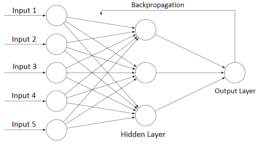Figure 1. The structure of MLP with Backpropagation algorithm

The backpropagation algorithm consists of two steps through the different layers of the network: forward step, an activity pattern (input vector) is applied thought the nodes of the network, and its effect propagates on the entire the network, layer by layer; and backward step, a set of outputs is produced as the actual response of the network, where the synaptic weights are all adjusted in accordance with an error correction rule [9].

In order to evaluate the performance measure in the neural network training process, was adopted the Mean Square Error (MSE), minimizing the MSE in the training set:

(1)

where N is the number of patterns in the data set, y_k is the true observational value, d_k is the estimation computed by the neural model, and E is the mean square error.

3.2. Self-configured MLP-NN

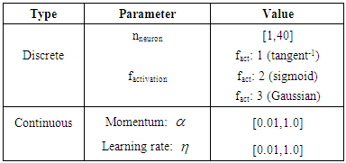
In recent years, the use of metaheuristics has been proposed as an efficient alternative to solve optimization problem. The optimal neural network topology can be expressed to minimize a cost function. Metaheuristics used to compute the best topology include hybrid Particle Swarm Optimization (PSO) and Genetic Algorithms (GA) [22], Constructive Method and Pruning [5], or applying severe algorithms: a comparison among Genetic Algorithm (GA), Simulated Annealing (SA), Generalized Extreme Optimization (GEO), and Variable Neighbourhood Search (VNS) [3].

Optimization problems have the goal of finding the best solution, finding an optimal value of an objective or cost function. Optimization problems can be classified as: continuous optimization (where the variable has real or continuous values); discrete optimization (where the variable has integer or discrete values); and mixed optimization (with integer and continuous values at the same time) [1].

In this paper, a technique for automatic configuration of neural network is formulated as a mixed optimization problem using MPCA algorithm.

The MLP topology is expressed by defining some parameters for the network: number of hidden layers, number of neurons for each layer, type of activation function, the learning rate, and the momentum constant.

3.3. Solving Optimization Problem by the MPCA

The MPCA was developed by Luz et al. [13], inspired from the canonical Particle Collision Algorithm (PCA) [20]. In the MPCA, a new characteristic is introduced: the use of several particles in cooperation, instead of only one particle moving in the search space. Both algorithms are inspired on two physical behaviors inside a nuclear reactor: absorption and scattering.

The PCA starts with a selection of an initial solution (Old_Config). The candidate solution is then modified by a stochastic perturbation (function Perturbation), leading to the construction of a new solution (New_Config). The new solution is compared with the old one (function Fitness), and the new solution can be accepted or not. If the new solution is not accepted, the particle can be sent to a different place in the search space, giving the algorithm the capability of escaping from a local optimum. This approach is inspired on the scattering process (function Scattering) – this issue can be considered as Metropolis’ strategy, see reference [14]. If a new solution is better than the previous one, this new solution is absorbed (function Absorption). The exploration around closer positions is applied by using the operators Perturbation{.} and Small_Perturbation{.} [13].

The implementation of the MPCA algorithm is similar to PCA, but it uses a set of N particles, where a mechanism for sharing the information among particles is employed – the cooperation feature. A blackboard strategy is adopted, where the Best_Fitness candidate is shared among all particles in the process. Results have shown that MPCA is able to compute good solutions, in which PCA cannot fiund good answers [13]. The MPCA is codified using Message Passing Interface (MPI) libraries on a multiprocessing machine with distributed memory.

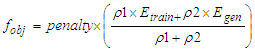
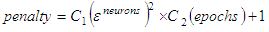
3.3.1. Objective Function

The objective function used in this study is a weighted average of two terms of square difference between the target values and the NN output, associated to a penalty term. The cost function is given by [3].

(2)

where ρ₁ = 1 and ρ₂ = 0.1, the same values proposed by Carvalho et al. [3]. These are adjustment factors for taking into account the relative relevance of training and generalization errors. The training error E_train provides a quantitative indication of the NN training level. The generalization error criterion E_gen is the ability of the NN to identify and respond similar standards based on the learned knowledge on new unknown examples/tasks after having experienced a learning data set.

The penalty term priorizes simpler topologies, avoiding the overfitting, using the number of neurons present in the intermediate layer (#neurons) and the total number of epochs (#epochs) to achieve convergence. The overfitting occurs when a NN begins to memorize training data rather than learning/extract information. The penalty is expressed as:

(3)

where C₁ = 1 and C₂ = 0.1 are adjustment parameters [3] for finding a good balance for the two factors in the complexity measurement.

The MPCA metaheuristic is used to compute four mixed-variable domain parameters: two continuous variables (the learning rate parameter, and the momentum constant) and two discrete variables (the number of neurons in the hidden layer (n_neurons), and the type of activation function (f_activation). The allowed values for these parameters are presented in Table 1.

Table 1. Parameters to define a neural network topology

3.4. Rough Set Theory

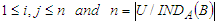
In meteorology, data from various sources (satellites, measurements from surface stations, ocean buoys, radiosondes, numerical models, devices for recording electrical discharges, radar, among others) are used for weather and climate prediction.

A technique for data reduction is proposed based on the Rough Set Theory (RST), to alternatively identify the input variables to the NN models for monthly and seasonal precipitation prediction.

Rough Set Theory (RST) was proposed in 1982 by Zdzislaw Pawlak as a mathematical theory to treat uncertain and imprecise information, by deriving approximations of a data set [16]. There are many formal models available for the treatment of uncertainties contained in database, such as Fuzzy Sets Theory [23]; Dempster-Shafer theory [7], and Possibility Theory [24].

The RST approach, applied in data analysis, requires no additional information on database, unlike other methods, as those mentioned above, such as the probability distribution, and the degree of pertinence [23]. Similar to the Fuzzy Set theory, the RST is an extension of classical set theory [16]. The fundamental feature behind RST is the approximation of lower and upper spaces of a set, the approximation of spaces being the formal classification of knowledge regarding the domain of interest.

Rough set theory can be considered as a specific implementation of imprecision expressed by a boundary region of a set, and not by a partial membership, like in fuzzy set theory.

A data set is represented as a table, where each row represents an object, and every column represents an attribute (a variable). This table is called Information Systems (IS), and is composed of a finite non-empty set U (Universe) of objects and a finite non-empty set A of attributes, IS=(U, A), such that , for every . A decision system (DS) is any information system, in which 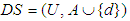, where is the decision attribute or conditional attributes [16].

3.4.1. Indiscernibility

The indiscernibility relation is used as a measure of similarity among objects, and it is considered a central concept in RST. Therefore, a set of objects with the same attributes are indiscernible, and cannot be distinguished from each other based on the available attributes [12].

Given IS=(U, A), then with any there is an equivalence relation associated :

(4)

where is the indiscernibility relation, and if two objects 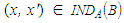, then objects x and x' are indiscernible one each other by attributes from B.

3.4.2. Set Approximation

In RST, the concept of the equivalence relation can be defined as a partitioning of the universe, where these partitions can be applied to build new subsets of the universe. Subsets that are most often of interest, have the same value of the outcome attribute [12].

For example, if it is possible to delineate objects that certainly have a positive outcome, or objects that certainly do not have a positive outcome and, finally, the objects that belong to a boundary between the certain cases. If this boundary is non-empty, the set is rough. These notions are formally expressed as follows.

The lower approximation of a set X with respect to B is the set of all objects, can be with certainty as members of X with respect to B, denoted (certainly X with respect to B).

The upper approximation of a set X with respect to B is the set of all objects which can only be classified as possible members of X with respect to B, denoted (possibly X in view of B).

The boundary region of a set X with respect to B is the set of all objects, which can be classified neither as X nor as not-X with respect to B.

3.4.3. Reduction

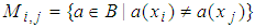
The reduction process is to identify the attributes that preserve the indiscernibility relationship [12]. Thangavel and Pethalakshmi [21] did a review of different methodologies to implement the RST strategy. The attributes representing discernible values are inserted into a matrix. Each entry in the matrix consists of a set of attributes that distinguish a pair of objects x_i and x_j as follows.

(5)

where .

The discernibility function for a subset B is constructed by concatenating the subsets M_i,j = {a*|a M_j,j}. The function determines the minimum set of attributes that distinguish any class among the existing classes and it is defined as follows.

(6)

where corresponding to the attributes.

Here, the Rosetta software package was used to perform dimensionality reduction of data – the system is available in the internet: http://www.lcb.uu.se/tools/rosetta [15].

4. Climate Prediction for Precipitation

The climate prediction is a set of natural conditions that dominate a particular region, obtained by the average behaviour of the atmosphere, employed to identify the atmospheric state in a future period of time (more than one month ahead).

Among the various outputs provided by weather and climate forecasting models, the precipitation is one of the meteorological variables of interest to society. Several tasks and decisions are dependent on such information, especially those related agriculture, hydroelectric power generation, transport and, civil defence.

Two models of MLP network were designed. One model was generated using all available variables in the database, and its topology as determined by solving the optimization problem (2) by using the MPCA metaheuristic. The other model with reduced number of variables indicated by RST was also self-configured by MPCA.

4.1. Meteorological Data

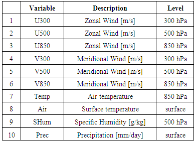
The data used in the experiments were obtained from the NCEP (National Center for Environmental Prediction) and NCAR (National Center for Atmospheric Research) databases. The reanalysis data embrace the entire planet with horizontal resolution (latitude x longitude) of 2.5° x 2.5° (see [11]), consisting of monthly averages for meteorological variables from Jan/1990 up to Feb/2015.

A data set is employed during the neural network training phase. The generalization capability from the ANN is tested by a set of validation data. Therefore, the verification data are divided into two subsets: examples and validation. The subset of examples is used in training the network. The training phase is interrupted periodically after a specified number of epochs, and the network is tested with the validation subset – the cross-validation process.

The generalization phase, a data set not used during the training phase, is presented to the ANN for evaluation and verification of the network performance.

From this consideration, the dataset was divided into three groups. The training data subset has data from January 1990 up to December 2010; the cross-validation data subset was created from January to December 2011 [11]; and the generalization test subset corresponds the period from January 2012 up to February 2015.

Table 2 provides a description of the meteorological variables selected from the NCEP/NCAR databases, with its units and levels (expressed at hPa), used in this study.

Table 2. Variables selected from the NCEP/NCAR

The climate prediction problem was applied into a selected subregion: with coordinates (Latitude 35S, 25S) and (Longitude 62W, 46W) in the South America. The considered regions are illustrated in Figure 2: see the red box – this includes Uruguay, Rio Grande do Sul and Santa Catarina Brazilian states, and part of the Paraná Brazilian state.

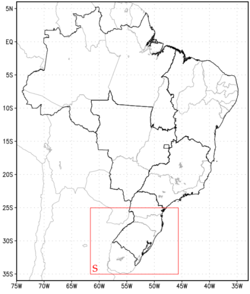Figure 2. Analysed area from the South (S) region of Brazil

The results were visualized using the GrADS (Grid Analysis and Display System) software. This software is available for free download: www.iges.org/grads/ [8].

4.2. Computational Experiments

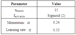
The weather and climate prediction uses sophisticated mathematical models to describe the behaviour of the atmosphere dynamics. These models are executed on a large computer system. CPTEC-INPE has the supercomputer Tupã: a Cray XT6 supercomputer with peak performance of 244 TFlops [4]. As already mentioned, all numerical experiments were carried out in the Tupã supercomputer, using 240 processors, with each processor having 12-cores.

The results from the MPCA are obtained after 15 executions. Each execution includes 500 different executions of the algorithm. The stopping criterion was considered the maximum number up to 500 objective function evaluations.

The precipitation prediction results were obtained using two different models of NNs: for the first model, the topology parameters were automatically determined by the MPCA metaheuristics. This neural network was trained using all variables available in the database (NN-all variables). For a second neural model, the precipitation prediction was obtained by a trained network with the reduced set of variables (NN-RST). This second NN has the same number of hidden layers (only one) with the same number of internal neurons as defined by the NN cited above. Table 3 shows the parameters for the optimal configuration of both neural networks (NN-all variables and NN-RST), as defined by the MPCA metaheuristics.

Table 3. Parameters obtained by MPCA

4.2.1. Reduction Meteorological Variable by RST

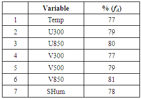
The variables that form the products have a presence greater than 70% in the discernibility function. It can be noticed that only 7 variables out of 10, were considered. The variables selected by RST are presented in Table 4:

Table 4. Parameters obtained by MPCA

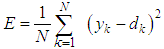
4.2.2. Error Analysis

Error maps for the precipitation prediction are computed from the difference between observation field (NCEP reanalysis) and precipitation prediction obtained by NN models. There are two prediction models: NN-all variables, and NN-RST. The error is calculated by:

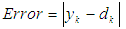(7)

where y_k is the reanalysis precipitation, and d_k is the precipitation prediction found by the neural network.

4.3. Monthly Precipitation Prediction

Figure 3 shows the monthly precipitation prediction results for the month at July 2014. Figure 3a shows the observed precipitation field at July 2014 extracted from the NCEP/NCAR database. Figure 3b and 3c are the precipitation prediction results obtained with two different NNs. The topology parameters were automatically determined by the MPCA metaheuristics. Figure 3b shows the result using all 10 variables shown in Table 2 (NN-all variables), and Figure 3c presents the precipitation predicted by the network trained with the reduced set of variables (NN-RST).

The results for July-2014 show that both NN models reached precipitation patterns similar to the reanalysis precipitation field. However, the NN-RST presented a lower error surface for Rio Grande do Sul and Santa Catarina States – see Figure 3e.

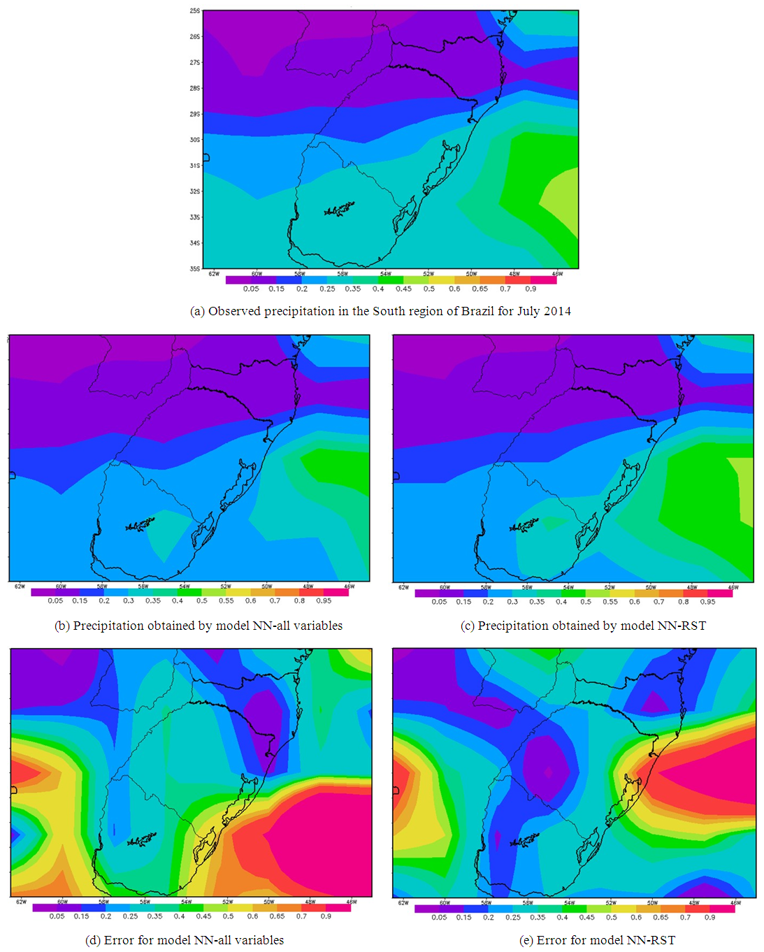Figure 3. Result for the monthly climate precipitation prediction for the South region of Brazil at July 2014. (a) shows the observed precipitation field extracted from the NCEP/NCAR database; (b) shows the results obtained by NN-all variables, that was design by MPCA, and was trained using all variables available; (c) precipitation obtained with NN-RST trained with a reduced set, and the topology was self-configured by MPCA; (d) shows the difference between observation field and precipitation prediction for model NN-all variables; and (e) error for model NN-RST, trained with a reduced set

4.4. Seasonal Precipitation Prediction

Figure 4 shows the seasonal precipitation forecast results for the winter season 2014. Figure 4a shows the precipitation field for winter season from the NCEP/NCAR database. Figures 4b and 4c are the precipitation prediction results obtained with different NNs: NN-all variable (using all variables shown in Table 3), and the NN-RST (variable shown in Table 4). Both neural networks were defined by the MPCA. Figures 4d and 4e show the error maps for the precipitation prediction using the models NN-all variables and NN-RST, respectively. Good predictions were obtained with both NNs.

The better prediction was found by the NN-RST – see Figure 4c – using the reduced set of variables selected by RST approach, as indicated by the error map in Figure 4e – error ranging in the interval [0.05; 0.5]. For this region, winter is considered as rainy season.

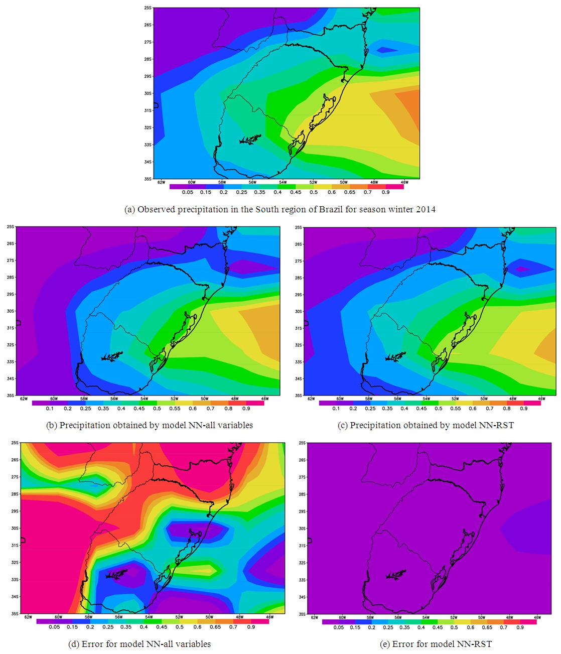Figure 4. Result for the seasonal climate precipitation prediction for the South region of Brazil in winter 2014. (a) shows the precipitation field extracted from the NCEP/NCAR database; (b) shows the seasonal precipitation result obtained by NN-all variables, that was design by MPCA, and was trained using all variables available; (c) presents the seasonal precipitation obtained by model NN-RST trained with a reduced set, and the topology was self-configured by MPCA; (d) shows the difference between observation field and precipitation prediction for model NN-all variables; and (e) error for model NN-RST, trained with a reduced set

5. Final Remarks

This paper addresses the climate precipitation prediction by using a neural network approach. Two climate time scales were considered: monthly and seasonal prediction. The neural networks were configured automatically, where the determination of the best neural network topology is formulated as an optimization problem. The MPCA meta-heuristic was applied to identify the best architecture for the neural networks.

The self-configuring scheme for the neural network produces not only the best topology, but the process also saves a lot of time from an expert for searching a satisfactory topology for a neural network. In addition, the methodology allows the use of a neural network approach for a larger audience.

Another contribution of this paper was the use of a data reduction method applied in the study of monthly and seasonal climate precipitation prediction, employing the theory of rough sets for data reduction, with focus on inputs for the neural networks as predictive models. The application here looks at the climate precipitation prediction in the Southern of the Brazil. The RST technique applied to the reduction of the data dimensionality allows the identification of relevant information in the data set employed to climate precipitation prediction without degrading the forecasting process. Furthermore, RST is a technique that deals with the problem of handling large amounts of data, which is characteristic in meteorology nowadays.

The neural prediction model produced good performance – see Figures 3b and 3c (monthly), and 4b and 4c (seasonal). The prediction carried out from the RST analysis was better than full input variables – see the error maps by Figures 3d and 3e (monthly), and 4d and 4e (seasonal). The latter result shows the relevance of data mining analysis.

Similar results are obtained by NNs for other months and seasons – not shown. For other seasonal predictions (Autumn, Spring, and Summer), the best results are also presented by NN-RST – as noted during the winter. For the monthly precipitation climate prediction, the NN-RST has also obtained a better performance for the other months in our experiments for 2014.

ACKNOWLEDGEMENTS

Authors want to thank the CNPq, CAPES, and FAPESP, Brazilian agencies for research support.