1. Introduction

One of the most important goals of operational forecasting is to predict the spatial and temporal characteristics of precipitation. Many socio-economic activities rely on precipitation knowledge, not only for lucrative or subsistence activities, but also to prevent natural disasters. Besides being an important variable, precipitation is also one of the most complex variables reproduced by numerical weather models. Microphysics and cumulus parameterization work together to produce precipitation in models of numerical weather prediction.

In southern Brazil, the precipitation is evenly distributed throughout the year [12] and [13], but the weather systems that generate the precipitation are different each season. In the autumn and winter, the cold front passage, associated with extratropical cyclogenesis are more frequent [10] and [5]. In spring and summer seasons, the occurrence of Mesoscale Convective Systems (MCS, as squall lines, Mesoscale Convective Complex – MCC, and daytime convection) is more frequent [16], [8], [18] and [1].

Studying the MCC (and the MCS in general) is important because the middle latitude of South America has been identified as an intense activity area of MCS [16], [8], [18] and [1]. According to [16], the MCC observed over South America have very similar characteristics to those observed over North America. That is, they develop preferentially during the night, on a flat area and present strong relationship with low level jet, but on average they are 60% larger than the MCC observed in North America. More recently, [3] analyzed 330 events in nine warm seasons and confirmed that in South America the MCC are larger and longer than in North America.

A good example of the difficulty of operational forecasting in predicting the correct precipitation distribution (spatial and temporal) generated by the MCC system can be seen in Figure 1. The MCC case hereinafter reported, developed between 11 and 12 July 2006 over the region between southern Paraguay, northern Argentina, Uruguay and southern Brazil. The observed accumulated rainfall showed two maxima, the most intense was located near 30°S-55°W and the other one, over the Brazil-Uruguay-Argentina border. Light rainfall was observed over Argentina and Uruguay. The operational forecasting (henceforth referred to as OPFOR) also showed two precipitation maxima, but they were positioned more to the northeast than the observed. The OPFOR just showed little precipitation over the northeast of Argentina and no rain over Uruguay. The secondary maximum of precipitation over the Brazil-Uruguay-Argentina border was not predicted by OPFOR. More details about the error in the precipitation operational forecasting, including the timing error, will be given in section 3.

Figure 1. Daily precipitation (mm) for 12 Jul for: (a) CPC analysis and (b) operational forecasting. Values of 1, 5, 15, and 30 mm are shaded

Thus, the aim of this study is to identify the reason for the low skill of the operational forecast. A few experiments were run in order to reproduce the precipitation pattern observed. Variations in the initial conditions, using another host model dataset, convective parameterization closure assumption type and the increase of horizontal resolution with nesting grid were tested. Section 2 presents the data and model used and the experiments conducted. Section 3 presents the spatial and temporal details of the precipitation field, and a discussion of the experiment runs. In the last section, the conclusions are presented.

2. Data and Methodology

The dataset used in this study are: GOES-12 IR channel satellite picture from DSA-CPTEC/INPE; automatic weather station network from INMET, CPTEC, Companhia de Geração Térmica de Energia Elétrica (CGTEE), and Agência Nacional de Águas (ANA); radiosonde data obtained from the MASTER-IAG/USP; daily gridded precipitation analysis for South America produced by the Climate Prediction Center (CPC) with resolution of 1° latitude x 1° longitude; and rainfall estimated by algorithm 3B42RT from Tropical Rainfall Measuring Mission (TRMM), which have a resolution of 0.25° latitude x 0.25° longitude.

For the initial condition and the host model three datasets were used: forecasting data form CPTEC/COLA Global Circulation Model (GCM), analysis from GCM (which is an analysis from the NCEP interpolated with GCM model grid) and analysis from GFS. The GFS analysis has horizontal resolution of 1° latitude x 1° longitude, 26 vertical levels and temporal resolution of 6 h. The horizontal resolution of the GCM analysis and forecasting is T126 (approximately 100 km), the vertical resolution is 14 levels and is available only at 0000 UTC and 1200 UTC for the analysis and each 6 h for the forecasting. The CPTEC/COLA GCM is a modified version of the spectral COLA GCM, which was adapted from NCEP GCM.

The model used in the operational forecasting and in the simulations was the 3.2 version of the Brazilian Regional Atmospheric Modeling System (BRAMS), which is the 5.04 version of the RAMS (Regional Atmospheric Modeling System) tailored for the tropics [4]. The main characteristics are [2] and [11]: 1) Arakawa-C grid stagger; 2) vertical coordinate shaved “ETA”-type, with 36 levels, initial spacing of the 100 m, 1.1 of the stretch ratio and maximum stretch limited in 1000 m; 3) shallow cumulus parameterization with Grell scheme [6]; 4) bulk microphysics parameterization [17]; 5) Chen and Cotton long/short-wave model; 6) Smagorinsky deformation-K closure scheme; 7) soil/vegetation/snow parameterization with LEAF3 model; 8) lateral boundary conditions with Klemp and Wilhelmson radiactive condition; 9) weekly observed SST, interpolated from 1° latitude x 1° longitude resolution dataset; and 10) homogeneous soil moisture specified in 40%.

All the experiments were run with BRAMS model, which is the RAMS adapted for the tropics. Nicolini et al. [9] showed that the RAMS is able to capture the strong forcing mechanism (low-level moisture convergence and upper-level divergence) favorable to organized convection, but it fails to produce enough precipitation or any precipitation at all.

Figure 2 indicates the grid domains (Grid 1 – G1 and Grid 2- G2), and the orography used in the experiments. Grid 2 is used as a nesting of G1 and covers a large part of Paraguay, northeast of Argentina, Uruguay and the south of Brazil. The orography is characterized by the Andes Cordillera (with elevations over 3000 m) in the west part of the model domain and the Serra Geral (with elevations between 500 m and 1000 m) in the eastern part of the domain (Figure 2). A large area with elevations no more than 250 m is located between these two mountainous areas (Figure 2). It is important to remark that the MCC development area is characterized by low elevation and absence of deep slopes.

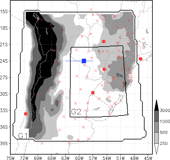Figure 2. Orography (meters, gray scale) used in the model. The grids used in the experiments (G1 e G2) are indicated in the lower left corner. Surface network (red “x” symbol) and sounding (closed red circle) station positions. The closed blue square and blue line in 24 oS refers to Figures 6a and 6b, respectively

All experiments began at 0000 UTC 11 July 2006 and ended at 1200 UTC 12 July 2006 with hourly output. Two horizontal grid configurations were used (Table 1). In the first experiment group, the operational forecasting grid configuration (called OPFOR), i. e., only one grid (G1) with 20 km of horizontal resolution was used. This configuration was used in 5 experiments (OPFOR, OPGCM, OPCON, OP12H and OP11L defined later). In the second group (experiments 2GOBS and 2GMCO), two grids were used (G1 and G2 grids), the first one with 40 km of horizontal resolution and the second grid with 10 km of horizontal resolution. In the experiments with two domains, grid 1 was configured to cover the same area covered as the grid with only one domain. The second group of experiments does not have an operational characteristic, because the data to insert in the initial condition are not available in real-time to perform operational forecasting. Moreover, these experiments could not be considered operational due to our available computational capacity. Anyway, the results are presented to complement the discussion on the most appropriate configuration for the operational precipitation forecasting.

Three different initial conditions were used (Table 1): i) GCM analysis used in the experiments OPFOR and OPGCM; ii) GFS analysis used in OPCON, OP12H, OP11L and 2GMCO, iii) GFS analysis modified to include the weather station network information is used in 2GOBS. This last option was conducted with Barnes objective analysis, which generated a new initial condition through the inclusion of 95 surface observations (indicated by red “x”) and 5 soundings (indicated by closed red circle), available in the region of the model domain at 0000 UTC 11 July 2006 (Figure 2).

Table 1. Characteristics of the operational forecasting and numerical simulations. P- Precipitation associated with the MCC

Another important aspect to point out is the host model data used as lateral boundary conditions (Table 1). The options used were: i) GCM analysis every 12 h in the OPGCM; and ii) GFS analysis every 12 h in the OP12H and every 6 h in the OPCON, OP11L, 2GOBS and 2GMCO. The GFS analysis rather than GFS forecasting was used as lateral condition because the GFS forecast might creat uncertainty in the BRAMS simulation. So, GFS analysis was chosen as a “perfect” forecasting and associate all the uncertainty to the BRAMS model. It is important to note that the GCM analyses are available only at two times (0000 UTC and 1200 UTC) and the GFS analyses are available every 6 h and with more vertical levels than the GCM analysis. In spite of the CPTEC/COLA GCM model running with 28 levels, only 14 vertical levels (1000, 925, 850, 700, 500, 400, 300, 250, 200, 150, 100, 70, 50 e 30 hPa) were used in the experiments in which the GCM (forecasting or analysis) provided the lateral boundary conditions. These levels were used because these are the levels available in the dataset for anonymous users. When the host model ran with the GFS analysis, the variables were disposed in 26 vertical levels (1000, 975, 950, 925, 900, 850, 800, 750, 700, 650, 600, 550, 500, 450, 400, 350, 300, 250, 200, 150 e 100 hPa), except for experiment OP11L in which only 11 vertical levels were used (1000, 925, 850, 700, 500, 400, 300, 250, 200, 150 e 100 hPa), which are the same levels than in the GCM dataset.

The cumulus convection is parameterized by the Grell [6] scheme, with the closure assumption given by 6 options: 1) standard Grell, 2) based on the omega velocity at cloud base, 3) based on the moisture convergence at atmospheric column (MC), 4) type like Fritsch-Chappel or Kain-Fritsch, 5) Arakawa-Schubert and 6) ensemble (EN, ensemble of the 5 previous closure types). All the experiments ran with the EN option, except for experiment 2GMCO that used the MC option (Table 1).

Two methods were used in the evaluation of the simulated precipitation, one subjective and the other objective. In the subjective method, it was considered that the precipitation associated with the MCC was well simulated when the precipitation generated by the experiment presented three characteristics: i) one area with rainfall rate between 0 and 1 mm/h at 0700 UTC 11 July; ii) this area enlarged and displaced to the south of Brazil; iii) the rainfall rate intensified, with intense precipitation (greater than 7 mm) over the extreme south of Brazil. The column labeled “P” in Table 1 was formed based on these three criteria, where the Yes word means that the precipitation associated to MCC was simulated and No, that the precipitation associated to MCC was not simulated. In the objective method (last column of Table 1), the Critial Succex Index (CSI, also known as Threat Score) was calculated between the simulated precipitation and the observed (CPC) or estimated (TRMM) precipitation.

3. Results

On the night of 10 July and the beginning of 11 July, a lower-level cloud area with temperature slightly lower than the land surface temperature was present over the north of Argentina and Paraguay (Figure not shown). These clouds moved southeastward, eventually located ending over the south of Paraguay and north Argentina at 0400 UTC 11 July (Figure 3a). At 0509 UTC 11 July these low clouds dissipated at the same time that convective cells developed (Figure not shown). These cells reached the maturity and dissipated at the same time that a new convective nucleus develops to the southwest as shown in Figure 3b-c. From this time on, the system acquired a circular shape (Figure 3d), displaced to the southeast (Figure 3e) and dissipated over the coastland (Figure 3f), where new nuclei developed firstly southeastward, over the east coast of South America and South Atlantic Ocean.

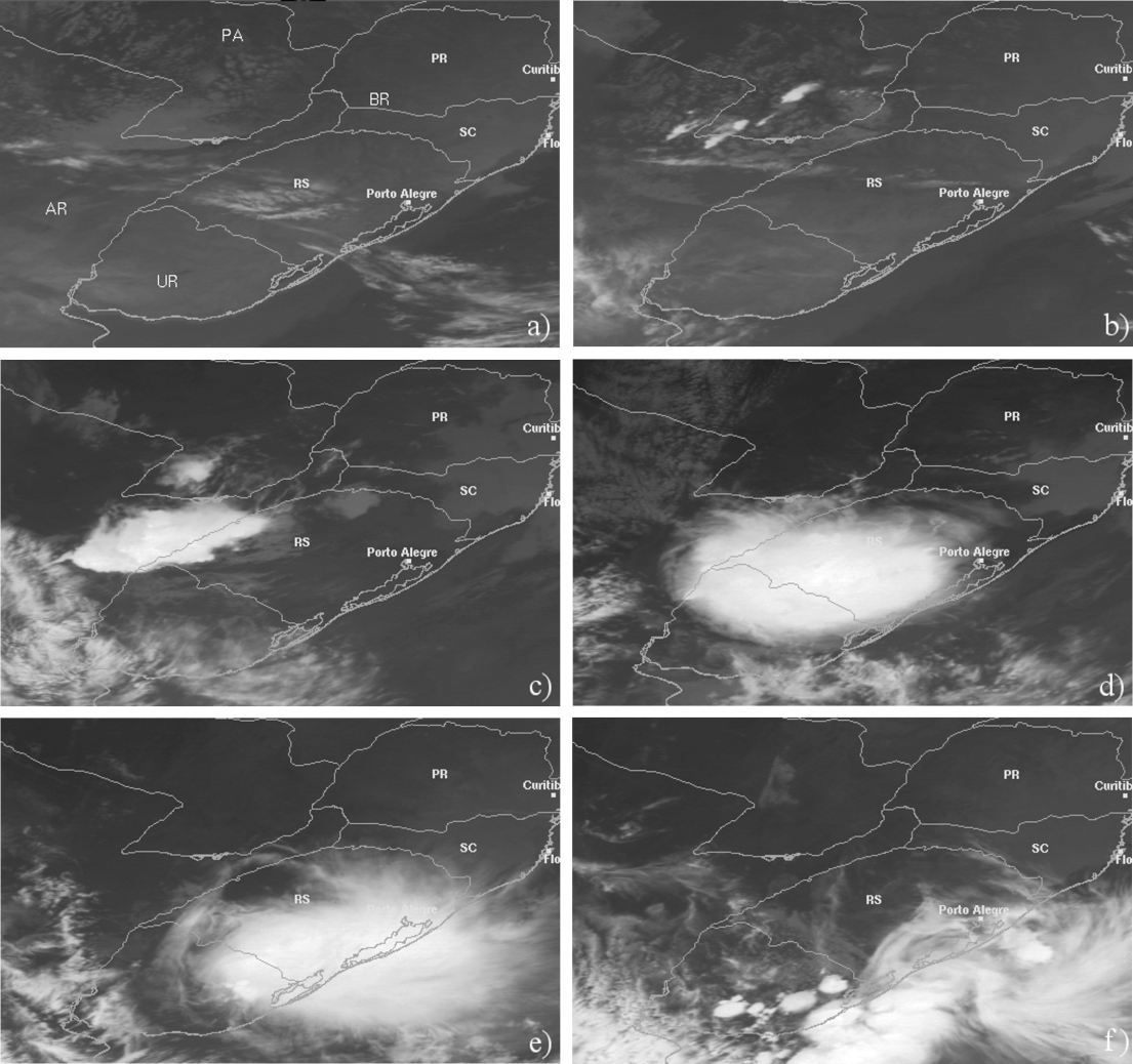Figure 3. IR GOES-12 satellite pictures for 11 July at: 0400 UTC (a), 0800 UTC (b), 1300 UTC (c), 1730 UTC (d), 2230 UTC (e) and at 0330 UTC 12 July (f). In Figure (a), the countries: Argentina (AR), Brazil (BR), Paraguay (PA) and Uruguay (UR), and the Brazilians southern states: Rio Grande do Sul (RS), Santa Catarina (SC) and Paraná (PR) are indicated

3.1. Spatial Precipitation Characteristics

The OPFOR 3 h accumulated rainfall between 2100 UTC 11 July and 0000 UTC 12 July is presented in Figure 4a. In the previous nine hours (at 1200 UTC to 2100 UTC), the precipitation was not forecasted, i. e., the precipitation on 11 July was forecasted from 2100 UTC on. The misplacement of the precipitation forecast can be observed in Figure 4a, where the weather stations that recorded precipitation (closed circle) and stations that did not record (open circle) are indicated. The spatial characteristics of precipitation are also noted in the TRMM data (Figure 4b).

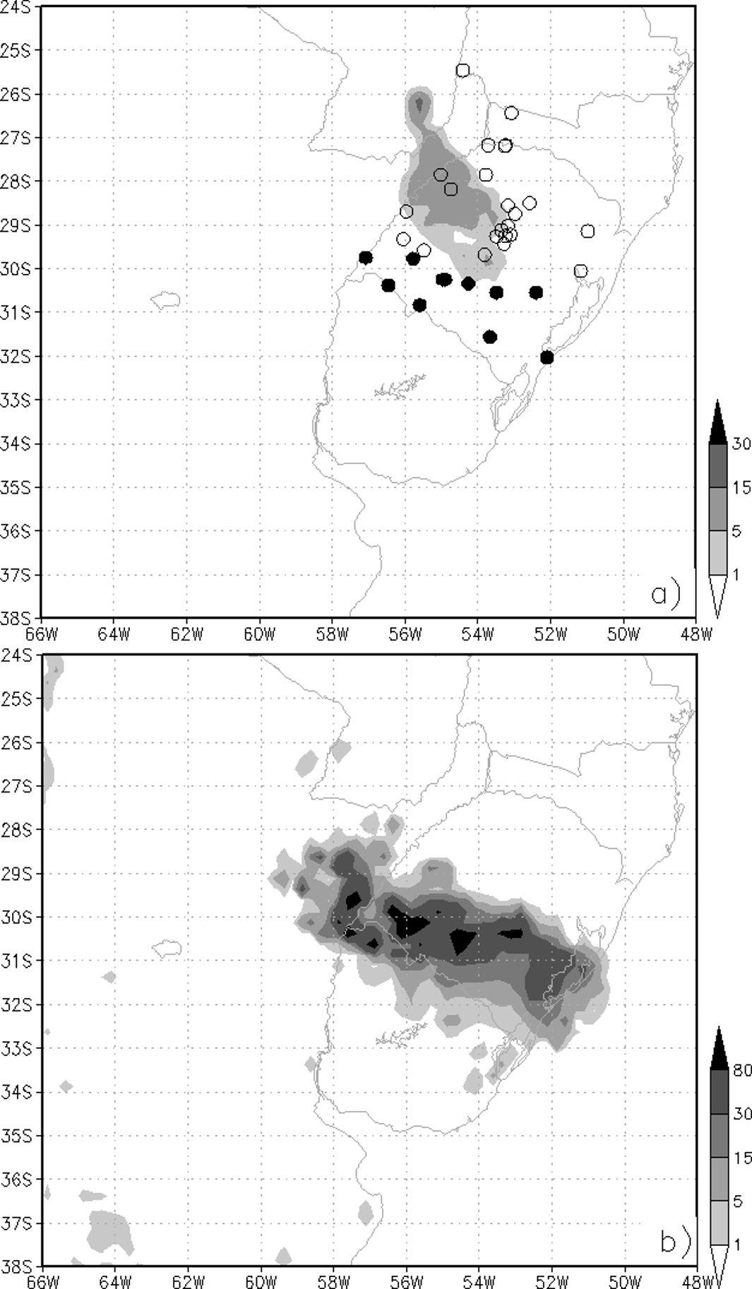Figure 4. Accumulated rainfall (mm) forecast between 2100 UTC 11 Jul and 0000 UTC 12 Jul, and the weather station positions (a). The closed circle indicates the weather stations which recorded rainfall; the open circle or square, stations with no precipitation recorded. Daily precipitation estimated by TRMM for 11 Jul (b)

From Figures 1a and 4, one can note that the OPFOR was not able to forecast the intense precipitation observed in the extreme south of Brazil, forecasting a precipitation band displaced more to the north than observed.

3.2. Numerical Simulations

As previously shown the OPFOR forecasted no rainfall over the north of Argentina and also produced a little quantitative precipitation over Brazil-Uruguay border. On the other hand, the OPFOR generated the rainfall displacement northward (Figure 1b, 4a). Based on the OPFOR configuration, some experiments were made by changing the following characteristics: i) the initial condition, by inclusion of the surface observations and sounding data; ii) closure assumption type for convective parameterization; and iii) soil moisture; but in neither change the precipitation associated to the MCC was simulated. Figure 5 shows the accumulated rainfall between 0000 UTC 11 July and 0000 UTC 12 July for some of the Table 1 experiments. In the OPGCM experiment, the model configuration was the same as in the OPFOR experiment, but with the host model given by GCM analysis each 12 h (0000 UTC and 1200 UTC times). Although the boundary condition was exchanged from forecasting to analysis (considered as “perfect” forecasting) data, the precipitation associated to the MCC continued not being simulated (Figure not shown) and the CSI remains small (CSI = 0.06 and 0.09, Table 1). The same happened with the closure assumption type change or with the horizontal resolution increase due to the second grid inclusion. Another experiment was conducted by changing the host model data (OPCON experiment). The OPCON experiment has the same OPFOR model configuration but the host model data are given by GFS analysis each 6 h. This simulation was able to start the convection over the south of Paraguay and north of Argentina and its posterior displacement to southeast over the extreme south of Brazil (Figure 5a) as seen in satellite pictures (Figure 3). Although the experiment simulated the precipitation associated to the MCC, it can be seen that the rainfall rate was lower than the observed. Also, the simulation trends displace the strongest precipitation to the north, without intense precipitation over the triple border Brazil-Uruguay-Argentina and Uruguay. The improvement of the precipitation pattern can be noted by the CSI which increased from 0.29 (for OPFOR) to 0.37 (for OPCON) for TRMM dataset (Table 1). Albeit the GFS data having a horizontal resolution similar to the GCM data, the GFS data have more vertical levels and are available every 6 h. The question placed is what defines the simulation of the precipitation associated to the MCC: the finer vertical resolution, the finer time resolution, or both?

Figure 5. Accumulated precipitation (mm, gray scale) between 0000 UTC 11 Jul and 0000 UTC 12 Jul for the same experiments listed in Table 1: OPCON (a), OP12H (b), 2GOBS (c) and 2GMCO (d). Accumulated rainfall is shaded for 0, 1, 5 and 10mm

It is interesting to remark that the precipitation associated with the MCC development happened with the GFS analyses as host model, but not with the GCM analyses. To analyze the hypothesis that the observation data absence at 0600 UTC and at 1800 UTC were essential to simulate the precipitation associated to the MCC, the experiment named OP12H was carried out with the same model configuration for OPCON experiment, but with host model updated each 12 h. In spite of the host model data given by GFS analysis, in this experiment the precipitation associated to the MCC was not simulated (Figure 5b). This was an unexpected result and it suggests that the 0600 UTC GFS analysis was essential to simulate the precipitation associated to the MCC.

Some studies for the South America area have shown that the low-level jet start and strengthen during the night, especially at 0600 UTC [14] and [7]. Thus, it seems that the BRAMS cannot simulate the low-level jet properly, making the inclusion of the lateral boundary conditions at 0600 UTC necessary. However, Saulo et al. [15], using the RAMS (precursor of the BRAMS), showed that the model can adequately represent the diurnal wind oscillation linked to planetary boundary mechanisms.

To verify the importance of the vertical levels in the GFS analysis, the OP11L experiment was run. In this experiment, the number of vertical levels was reduced to 11. With the same levels available in the GCM datasets (forecast and analysis) below the 100 hPa level. All the model configurations of the OP11L experiment were the same as the OPCON one. As suspected, the precipitation associated to MCC was not well simulated (Figure not shown, Table 1) when the vertical level number was reduced. The CSI decreased from 0.37 (for OPCON) to 0.09 (for OP11L) in relation to TRMM dataset. It is supposed that with 26 vertical levels, the lower troposphere was well represented, because in the OP12H experiment 12 levels below 500 hPa were available, while in the OP11L experiment only 4 levels were. The greater quantity of levels below 500 hPa tends to improve the PBL evolution, which is important for the MCC formation and evolution.

The effect of the complete GFS dataset can be seen in Figure 6. The vertical profile of the moisture convergence at 0600 UTC 11 July (time of the genesis of the MCC) shows that in the OPCON and OP12H experiments there was stronger moisture convergence in the lower troposphere than in the OP11L experiment (Figure 6a). This can be related with the fact that in the two former experiments the GFS dataset was thoroughly used, and in the later experiment, some lower levels were removed. Although the lower troposphere moisture convergence (Figure 6a) and moisture flow (Figure 6b) in the OPCON and OP12H experiments were similar before or during the MCC genesis, the moisture flow decreased with time and became similar to the OP11L experiment. This suggests that the complete GFS analysis is necessary to maintain strong moisture flow and moisture convergence in the lower troposphere.

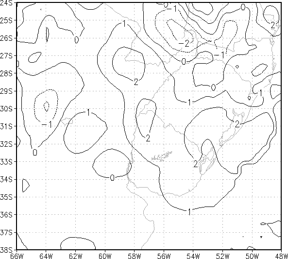
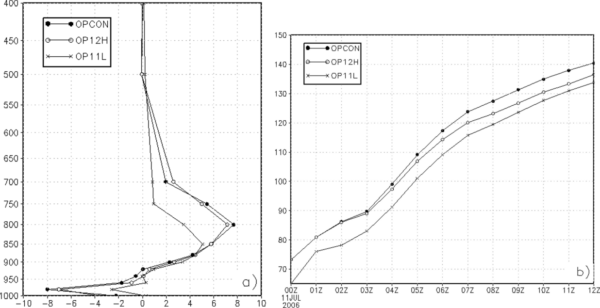Figure 6. Vertical profile of the moisture convergence in 24°S and 59°W (closed blue square in Figure 2) at 0600 UTC 11 Jul (a) and moisture flow vertically integrated (from 1000 hPa to 700 hPa) over the latitude of 24°S, form 63°W to 57°W of longitude (blue line in Figure 2) to: OPCON (closed circle), OP12H (open circle) and OP11L (closed square) experiments

Aiming improve the precipitation simulation associated to the MCC, other experiments were made changing the horizontal resolution, the initial condition and the convective parameterization closure assumption type. To form the 2GOBS experiment, the OPFOR configurations were changed to: i) the inclusion of a second grid to increase the horizontal resolution (from 20 km to 10 km); and ii) the initial condition changed by adding the observations (station nudging). The initial condition change was idealized considering the observational data available in the operational forecasting routine, and that the failure in the MCC prediction could be caused in part, by the erroneous initial condition. The inclusion of observational data generated notable changes in the surface meteorological fields and generated a better precipitation spatial distribution (Figure 5c, which must be compared with OPCON experiment in Figure 5a). The improvement of precipitation spatial distribution can be observed over the northeast of Argentina and in the south sector of southern Brazil, and by the increase of CSI to 0.54 (for 2GOBS) compared to 0.46 (for OPCON) in relation to CPC dataset (Table 1). However, the tendency to generate intense precipitation to the north (over the north area of southern Brazil) still persists. The effect of the surface observations can be noted in the lower temperature over the southwest quadrant of the domain where the consequent displacement to the southwest of the stronger surface temperature gradient (Figure not shown) and higher surface moisture content over the interest region (Figure 7) is observed. With relation to moisture field, Nicolini et al. [9] noticed that the NCEP reanalysis also provide insufficient surface moisture content when compared with the observed values.

Figure 7. Difference of the vapor mixing ratio at 2 m above ground 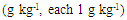between analysis plus observation and analysis only at 0000 UTC 11 Jul

The last experiment (2GMCO) was presented to get the major precipitation quantity at the triple border and in the Brazil-Uruguay border (Figure 5d). This experiment presented the same configuration as the 2GOBS experiment, except that the initial condition is given by GFS analysis only and the convective closure assumption type was changed to the MC option (Table 1), i. e., the closure was based on the moisture convergence at the atmospheric column. This experiment showed a higher quantity of precipitation in the direction of the Brazil-Uruguay border and less in the north part of south Brazil. These characteristics indicate some improvement in spatial distribution of precipitation, as also is suggested by the CSI value that increased from 0.37 (OPCON) to 0.39 (2GMCO) with relation to TRMM dataset (Table 1). But the secondary precipitation maximum observed at the triple border did not continue to be generated. The rainfall rate at every 2 h for the 2GMCO experiment shows that the precipitation started at 0600 UTC 11 July (0611) over the Argentina-Paraguay border (Figure not shown), displaced southeast (Figure 8a-e) and became more intense over the Argentina-Brazil border (Figure 8f-g), as suggested by the satellite image (Figure 3), and TRMM data (Figure 4b).

Figure 8. Rainfall rate (, gray scale) in 2GMCO experiment for grid 2, began at 0800 UTC 11 Jul (a) and ended at 0000 UTC 12 Jul (i), at intervals of 2 h. The values between 0, 1, 3 e 6 are shaded. The numbers in the upper left corner indicate the hour and day of Jul 2006. For example, 0811 indicates the 0800 UTC 11 Jul

The experiments resulted in different precipitation characteristics, but all experiments showed that the rainfall magnitude was underestimated when compared with TRMM estimates (Figure 4b) and surface observations (Figure 1a). Moreover, the accumulated rainfall was oriented in the northwest-southeast direction in all the experiments. In the TRMM estimates and the pattern derived from surface observation, on the other hand, the orientation presented a smaller northwest-southeast direction tilt.

4. Conclusions

In this study the reason why a MCC case was not very well forecasted with an operational forecasting system is analysed. The MCC formation occurred over southern Paraguay and northern Argentina around 0600 UTC 11 July 2006 and displaced southeastward in direction of the extreme south of Brazil, generating intense precipitation over the region. To determine why the skill of the numerical precipitation forecast was low, a set of experiments with some changes in the operational forecasting configuration were realized. The modifications were: i) the host model data, and ii) model configuration.

From the experiments performed, it can be concluded that a better temporal and vertical resolution is essential to simulate the precipitation associated to the MCC resided in the GFS data. Thus the inclusion of the analysis at 0600 UTC 11 July, even though there was no SYNOP data over Brazil but with surface data over Argentina and Paraguay, which covered a large part of the initial the MCC development area. It is noteworthy that using the GFS analysis as host model and excluding the analysis at 0600 UTC 11 July, the development of precipitation associated to the MCC was not very well forecasted. The same happened when the vertical level number was reduced in the GFS data. Thus, it supposed that the OPFOR was dominated by the moisture convergence area established throughout the latitude of 27^oS located over the northeast of Argentina and the south of Brazil at 0000 UTC 11 July (in initial condition), generating intense precipitation dislocated northward, which does not allow the MCC formation at 0600 UTC 11 July. Meanwhile in the observation analysis there was an established intense moisture convergence area located over the Paraguay and Argentina border.

With the GFS analysis as the host model and using the operational forecasting model configuration it was possible to simulate the precipitation associated to the MCC; however, the accumulated precipitation located northward of the observation data was inferior to the observed one. In this way, the simulations were carried out with some modifications in the model configuration to displace the accumulated precipitation southward. The configuration of the best results was as follows: i) two grids, the first one with 40 km and the second with a 10 km horizontal resolution; ii) inclusion of surface weather station and radiosonde observations to improve the initial condition at 0000 UTC 11 July; and iii) exchange of convective parameterization closure type to moisture convergence. With these configurations, it was possible to simulate higher quantity of precipitation displaced to the Brazil-Uruguay border, and with the intense precipitation over the extreme south of Brazil. Although the simulated precipitation was greater, the intensity was still smaller than the observed. The secondary accumulated precipitation maximum over the triple Brazil-Uruguay-Argentina border was not simulated by any experiment realized.

Finally, it can be concluded that for this specific case, it might be possible to get an acceptable operational forecast of the MCC through: i) from a more appropriate model configuration; ii) an assimilation data scheme that include the observation data of 0000 UTC and 0600 UTC times; and iii) with a host model provided with more vertical level number, mainly below 500 hPa level. The optimal configuration should have the following characteristics: i) two grids, the first with 40 km and the second with 10 km; and ii) the deep convective parameterization closure assumption based on the moisture convergence at atmospheric column.

ACKNOWLEDGEMENTS

The research reported in this paper was carried out with the support of CAPES (Project 7920) and CNPq (Project 381246/2007-8), entities of the Brazilian Government directed toward the formation of human resources and scientific and technological research. Thanks to DSA-CPTEC/INPE, INMET, MASTER-IAG/USP, CGTEE, for allowing free download of all dataset used in this study.