1. Introduction

It is common knowledge that the General Circulation Models (GCMs) are not able to display a resolution fine enough to resolve small-scale atmospheric circulations, such as circulations affected by the orography, ocean proximity or characteristics of the surface of the earth. Consequently, many of these models have shortcomings that limit seasonal climate simulations. In this sense, many studies point out the deficiencies of GCM in climate prediction (e.g., [1]; [2]; [3]; [4], among others).

An alternative to improve and reproduce climate simulations in detail is the use of limited-area models.The use of this technique has led to many studies, e.g., [5]; [6]; and [7]. Such models nested within GCMs are called Regional Climate Models (RCMs) and are forced by the lateral boundaries provided by the GCM. Even though GCMs solve large-scale systems, as those responsible for the variability in temperature and precipitation, they do not solve sub-grid scale processes due to its coarse resolution. The GCMs are not sufficient to assess climate changes [4] caused by complex surface characteristics. The RCMs, on the other hand, consider sub-grid scale processes, such as topography, land-ocean and vegetation contrasts, and thus can reproduce a regional climate pattern closer to reality. Some parameterizations includeding these models can be advantageous, such as in achieving a better resolution of the sub-grid orographic precipitation.

Southern Brazil is in a transition region between the summer monsoon regime and winter conditions of mid-latitude. Since Rio Grande do Sul is the southernmost state of Brazil, and the one that better represents the mid-latitude systems, it will be the focus of analysis of this study.

The need for long-term climatologies is evident because it provides basic conditions to assess seasonal predictions. However, [8] the authors of reference emphasize that an ensemble of multiple models is required to characterize the inherent uncertainties.

In this work, nine simulations using different cumulus parameterization schemes available in the Regional Climate Model RegCM4 were carried out and evaluated in order to simulate climatological temperature from 1974 to 2005. Additionally, we tested new convective parameterizations discussed by [9], who suggest land/ocean mixed parameterization.

2. Materials and Methods

In order to make seasonal forecasts, we used the RegCM model [10] and [11], that originated in NCAR (National Center for Atmospheric Research) from the Mesoscale Model version 4 (MM4, [12]). The first version of the model, RegCM1, was developed in 1989 and since then has undergone major upgrades in 1993 (RegCM2), 1999 (RegCM2.5), 2006 (RegCM3), and most recently, 2010 (RegCM4).

This version includes important enhancement in the code structure, pre-and post-processing, and inclusion of new physical parameterizations. The model is flexible, portable and easy to use. It can be applied to any region of the world, with a spacing grid up to about 10 km (hydrostatic limit), and to a wide range of studies, from paleoclimate processes to simulation of future climate scenarios. Ongoing improvements include a tropical band version, the coupling to a regional ocean model, incorporation of full gas-phase chemistry, updates of some physical schemes (convection, PBL, microphysics cloud model), and the development of a non-hydrostatic dynamic core [13].

2.1. Cumulus Parameterization

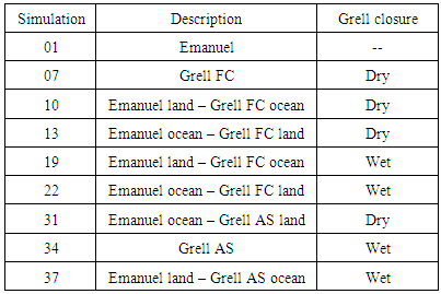
The cumulus convection plays an essential role in the general atmospheric circulation. Due to their horizontal resolution of the order of hundreds of kilometers or more, the GCMs can not resolve the cumulus clouds, which have diameters ranging from 1-10 km. The representation of cumulus in terms of sub-grid is called cumulus parameterization.

Reproduction of atmospheric circulation in numerical models is extremely sensitive to formulation of cumulus parameterization [14]. In general, the cumulus convection modifies the large-scale temperature and moisture field through disentangling and cumulus-induced environmental subsidence. The former causes large-scale cooling and moistening, while the latter causes large-scale heating and drying [15].

Nowadays, there are several schemes developed for the parameterization of cumulus clouds. This work will use the schemes developed by Grell [16] and MIT-Emanuel [17] and [18].

The Grell scheme starts when a parcel of air is lifted and reaches the Lifting Condensation Level (LCL), becoming saturated. The condensation in the updraft is calculated by lifting a saturated parcel. In downdraft, mass flow depends on the ascending current, since the mass flow should be constant within the cloud. Two closing hypotheses can be used in this scheme: Arakawa and Schubert - AS [15] and Fritsch and Chappell – FC [19]. This closure is used to determine the modulation of the convective environment, being the dynamic control in Grell’s parameterization scheme [16].

The MIT-Emanuel system is triggered when the equilibrium level is greater than the cloud base level. When this occurs, afraction of air is lifted and a part of the moist air in this fraction condenses to form precipitation, while the remaining fraction consists on the cloud. Besides being a more complex representation of convection, Emanuel’s scheme includes in its formulation the self-conversion of the cloud water into precipitation within the cumulus clouds, which considers the appearance of ice, turning self-conversion into a temperature dependent process.

Table 1 shows the execution set ups for the climate rounds being carried out.

Table 1. Parameters of the simulations performed

2.2. Input Data and Domain

Model initial and lateral boundary conditions were created with the NCEP/NCAR Reanalysis II Project (NNRP) [20]. NNRP2 is derived from various data sources including radiosondes, surface marine data, aircraft data, surface land synoptic data, satellite sounder data, special sensing microwave imager, and satellite cloud drift winds. Quality control studies are performed and the data is assimilated using a numerical prediction model. SSTs were obtained from the NOAA optimum interpolation (OI) SST analysis (Version 2) [21]. In many regions where observations are sparse, particularly in the tropics, the NNRP2 dataset is more model dependent.

These data have horizontal resolution of 2.5° x 2.5° (latitude x longitude) and are available every six hours (00:00, 06:00, 12:00, 18:00 UTC). For the simulations, we used temperature, geopotential height, zonal and meridional wind and relative humidity data at 18 vertical levels of pressure. The period assessed was from 1991 to 2009. We built a nineteen-year precipitation climatology for each existing convective scheme in the model and thus we can determine what parameterization best reproduces the characteristics of Rio Grande do Sul.

2.2.1. Surface Data

The topography and types of soil cover used in RegCM4 simulations employ global files with a 10-minute resolution provided by the USGS (United States Geological Survey) and by the GLCC (Global Land Cover Characterization), which interpolated with RegCM provide the land boundary conditions. More information on the GLCC data can be found in http://edcdaac.usgs.gov/glcc/glcc.html.

2.3. Domain and Horizontal Resolution

The resolution was set at 50 km, with 60 grid points in the x direction, 40 grid points in the y direction, and 18 vertical sigma levels. The domain used in the simulations include the Latitudes of 35 S – 22 S and Longitudes of 66 W – 39 W, centered on 30 S, 53 W (Figure 1).

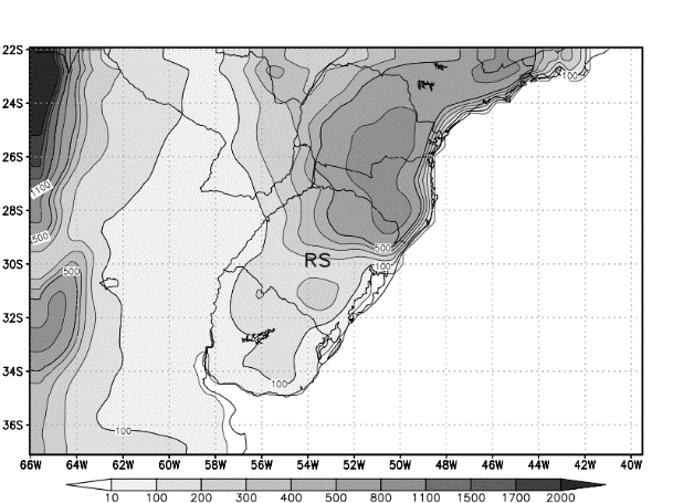Figure 1. Domain and topography in meters (m) used in numerical simulations

3. Results and Discussion

Initially, we compare the spatial pattern simulated with the climatology observed, generated by the National Institute of Meteorology (INMET). As an example, Figure 2 shows two months of climatology generated by the simulation 10 (a-summer and b-winter). Additionally, two months of climatology generated by the INMET from observational data are presented. It is possible to notice the closes patial and numerical agreement between modeled and real data. The model captures the east-west temperature gradient in the summer. The minimum values found in the mountainous region of RS (Northwest), around 20 °C, are also observed in the simulation. In the winter, the temperature gradient has a northwest-southeast displacement with higher values in the Northwest of the state. Again, this pattern was well simulated, including the cold air intake in the Southeast region.

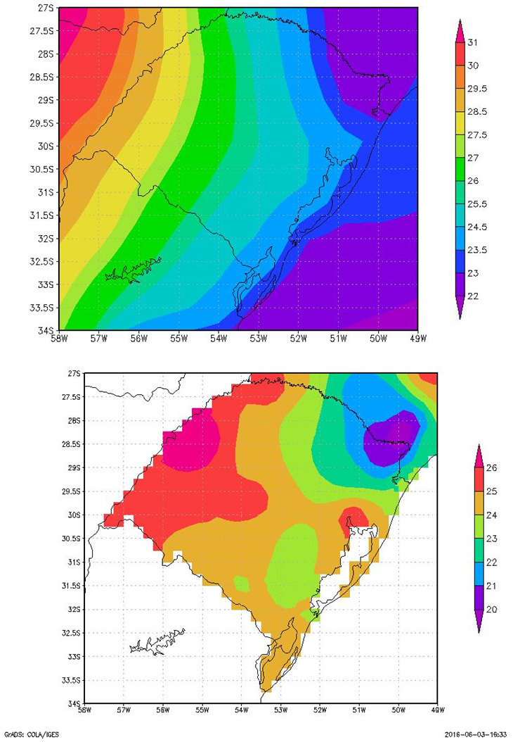Figure 2a. Climatology for January (top) andINMET climatological normal (lower) for the same period - right

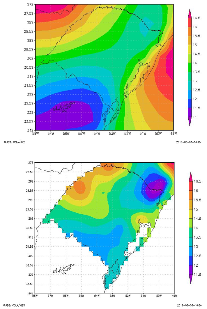Figure 2b. Climatology for July (top) and INMET climatological normal (lower) for the same period - right

In order to numerically evaluate the predictions, we calculated the Taylor diagram (Figure 3). In the diagram, each set of data is represented by a point, which is defined as the correlation values, standard deviation and root mean squared error. The closer the points are, the greater is the degree of similarity between them. The standard deviation is proportional to the radial distance to the origin.

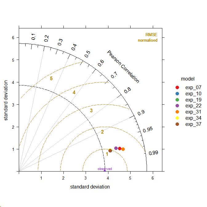Figure 3. Taylor diagram for the observed mean temperature (purple circle), and for the seven parameterization used (colored as the caption to the right)

It can be noticed that the standard deviation of the observed data is slightly lower than 4°C/month. The data generated by RegCM is very similar to the real data (around 4°C and 5°C/month), and the exp_37 gives the values closest to the actual standard deviation. The correlation coefficient of data generated by RegCM model is very close to 0.97. For this amount of data, any correlation value above 0.48 is statistically significant at a level of 95% according to the Student’s t test. The normalized mean squared error (which is the difference between the simulated and observed values) is proportional to the distance from the point on the x-axis labeled as “observed”. The variation is approximately 4°C/month.

These results show that for the variable temperature, all simulations yielded results very similar to the real ones.

When evaluating the annual cycle of climatology for each of the simulations, we observe that the annual pattern, with lower temperatures in June and July and higher in December to February, is well simulated. However, the RegCM has a tendency to overestimate the temperature in the hot season.

Regarding the average of the 7 experiments, there is a greater correlation between the observed and simulated data. In figure 5, a scatterplot of the average of the 7 experiments and the observed data is shown. The lower limit of average temperature is roughly the same for both sets, and the upper limit of the simulated temperature is about 2°C higher than the average of the observed temperature, what agrees with the evaluation of months when considered individually (Figure 4). [22] The authors of references found that for different regions of Central America, climate simulations with parameterization of cumulus clouds can generate temperatures with positive or negative bias. Therefore, there is a strong dependence of the simulation in relation to the dominium employed.

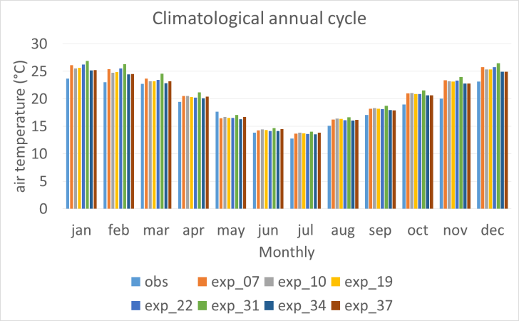Figure 4. Climatology of annual cicle

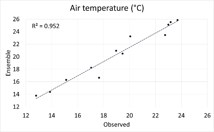Figure 5. Dispersion between the temperature observed and the average of the 7 experiments

4. Conclusions

The performance of the regional model RegCM4 was evaluated for a 20-year simulation of the average temperature for the state of Rio Grande do Sul, using seven different parameterizations of cumulus clouds. Summer and winter temperature patterns were well represented by simulation 10 (Emanuel land- Grell with Fritsch & Chappell ocean). Both the east-west temperature gradient in the summer and the north-south in the winter, as well as the extreme values of the mountainous region, have been identified. A similar behavior appears in all omitted parameterizations. The pattern of high temperatures during the summer and low temperatures during the winter is also well represented by all simulations, what explains the high correlation values observed. Furthermore, an improvement in the simulation of the temperature is obtained when using an average of all experiments. A further analysis shows that the simulation with Emanuel on earth - Grell Arakawa and Schubert on ocean (37) is the one with the best results.

ACKNOWLEDGEMENTS

We thank the weather and climate physics group of theinternational center for theoretical physics for providingthe RegCM. The second author gives special thanks to CAPES for MSc scholarship and the first author thanks FAPERGS for the financial support (PROMEM project).