-
Paper Information
- Paper Submission
-
Journal Information
- About This Journal
- Editorial Board
- Current Issue
- Archive
- Author Guidelines
- Contact Us
American Journal of Environmental Engineering
p-ISSN: 2166-4633 e-ISSN: 2166-465X
2016; 6(A): 56-65
doi:10.5923/s.ajee.201601.09

Derivation of a Decorrelation Timescale Depending on Source Distance for Inhomogeneous Turbulence in a Shear Dominated Planetary Boundary Layer
 Abstract
 Reference
 Full-Text PDF
 Full-text HTML
Franco Caldas Degrazia 1, Gervásio Annes Degrazia 2, Marco Tullio de Vilhena 3, Bardo Bodmann 3
1Environmental Engineering Department, Centro Universitário Ritter dos Reis – UNIRITTER, Porto Alegre/RS, Rua Orfanatrófio, Brazil
2Physics Department, Federal University of Santa Maria, Santa Maria/RS, Campus Universitário, Prédio 13 CCNE, Brazil
3Mechanical Engineering Graduate Program (PROMEC), Federal University of Rio Grande do Sul – UFRGS, Andar, Brazil
Correspondence to: Franco Caldas Degrazia , Environmental Engineering Department, Centro Universitário Ritter dos Reis – UNIRITTER, Porto Alegre/RS, Rua Orfanatrófio, Brazil.
| Email: |  |
Copyright © 2016 Scientific & Academic Publishing. All Rights Reserved.
This work is licensed under the Creative Commons Attribution International License (CC BY).
http://creativecommons.org/licenses/by/4.0/

In the literature there exists a variety of pollution of dispersion models and in general, Lagrangian stochastic models are efficient and fundamentals tools in the investigation and study of turbulent diffusion phenomenon in the planetary boundary layer. The LAMBDA model is one of them. In this study, the influence of decorrelation time scales in the LAMBDA model under neutral conditions is evaluated. To this end a new parameterization of decorrelation time scales is proposed and validated. This method is based on the Eulerian velocity spectra and a formulation of the evolution of the Lagrangian decorrelation timescales. A spectral distribution of an Eulerian velocity profile and a formulation of the evolution of Lagrangian decorrelation timescales under neutral conditions is used as the forcing mechanisms (shear-dominated boundary layer) for the turbulent dispersion. The model performance was established by comparing the levels of ground-level concentrations of the tracer gas with experimental results from the classical Prarie Grass experiment.
Keywords: Planetary boundary layer, Turbulent eulerian velocity variance spectra, Shear-dominated boundary layer, Lagrangian decorrelation time scales
Cite this paper: Franco Caldas Degrazia , Gervásio Annes Degrazia , Marco Tullio de Vilhena , Bardo Bodmann , Derivation of a Decorrelation Timescale Depending on Source Distance for Inhomogeneous Turbulence in a Shear Dominated Planetary Boundary Layer, American Journal of Environmental Engineering, Vol. 6 No. A, 2016, pp. 56-65. doi: 10.5923/s.ajee.201601.09.
Article Outline
1. Introduction
- Dispersion and transport models of contaminants are useful tools to evaluate anthropogenic influences in the environment. Actually, there are different kinds of dispersion models and in general, Lagrangian stochastic models are efficient and fundamentals tools in the investigation and study of turbulent diffusion phenomenon in the planetary boundary layer. The Lagrangian dispersion model LAMBDA [9] is one of them. In the stochastic Lagrangian model the turbulent dispersion was stablish by the particle movement of the fluid flow. This kind of model represent eddy motions where the particle velocities are subject to random forcings [22]. In this case, for each time step, the fluid particle moves due to the action of a mean wind and turbulent diffusion. The latter is caused by the action of wind velocity fluctuations. The Langevin equation solution is a continuous stochastic Markov process [23]. The position of the particle and its speed in a turbulent flow may be considered turbulent Markov processes in the energy range of the spectrum. This spectral range is between the velocity correlation Lagrangian scales (energy-containing eddies), and dissipative Kolmogorov timescales (eddies in which the molecular diffusivity acts strongly). In a stochastic Lagrangian model, applied to the simulation of the dispersion of a turbulent flow, the simulated trajectory of each particle represents an individual statistical realization of the flow. This flow is characterized by certain initial conditions and physical constrains. As a result, the movement of any particle is independent of other. Thus, the concentration field, i.e. the estimated spatial distribution of particles, should be interpreted as an average, performed over the total number of simulated particles [24]. Finally, in this study the model LAMBDA was employed to simulate the contaminant concentration field. This model employs a Gaussian distribution function for the horizontal probability directions. In the vertical direction, the probability function is not Gaussian. Such distribution functions are used to solve the Fokker-Planck equation, which provides the parameters that describe the stochastic Lagrangian model. Several studies of modeling dispersion of contaminants have used parameterizations of eddie diffusivity that are employed in analytical air pollution models in distinct atmospheric stabilities. Ref. [1] had success in the use of eddie diffusivity depending on source distance, in a shear dominated planetary boundary layer. An analytical solution of advection–diffusion equation called 2D-GILTT was used. Ref. [2] also tested parameterizations of vertical time dependent eddie diffusivity with a GILTT analytical model to solve the advection–diffusion equation. The authors of ref. [5] proposed a general formulation for pollutant dispersion in the atmosphere by using an arbitrary vertical profile of wind and eddy-diffusion coefficients considering local and non-local turbulence closure. A general analytical formulation for pollutant dispersion in the atmosphere was used by solving the time-dependent three-dimensional advection–diffusion equation by the combination of Laplace transform technique and the generalized integral advection–diffusion multilayer technique. Differently to the Eulerian dispersion models and the GILTT, ref. [8] presented a turbulence parameterization for the planetary boundary layer (PBL) dispersion models in all stability conditions. The tracer dispersion was simulated by the Lagrangian particle model LAMBDA [9, 10].Thus, the aim of this study is evaluate the model LAMBDA with different turbulent parameterizations. Hence, a formulation of the evolution of the Lagrangian decorrelation timescales under neutral conditions is derived and applied as forcing mechanisms (shear-dominated boundary layer) for the turbulent dispersion.
2. Derivation of Lagrangian Decorrelation Timescales
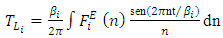
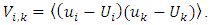
- The present approach basically hinges on Batchelor’s time-dependent equation [20] for the evolution of the Lagrangian decorrelation timescales

 | (1) |
 is the Eulerian energy spectrum normalized by the Eulerian velocity variance
 is defined as the ratio of the Lagrangian to the Eulerian integral timescales, n is the frequency, and t the travel time. By virtue Eq. (1) contains
  thus it describes
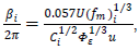
  from a Lagrangian perspective too, and Eq. (1) expresses a Lagrangian decorrelation time scale in terms of the ratio of the Eulerian energy spectrum to the Eulerian vertical velocity variance.It is well known that turbulent dispersion in the neutral PBL is generated by mechanical processes and is related to wind shear, and it is most effective close to the ground. This forcing mechanisms produce a wide range of scales (eddies) with infinite degrees of freedom. The present approach arises from the Eulerian velocity spectra under neutral conditions and can be described as a function of shear driven PBL scales [1]:
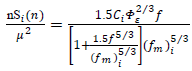 | (2) |
 and 4/3 for the
  and
and  components respectively [4];
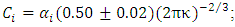
  is the von Karman constant,
  is the dimensionless frequency
  being the cyclic frequency,
  the mean horizontal wind speed and
  the observation height),
  is the dimensionless frequency of the neutral spectral peak and
  is the local friction velocity for a neutral PBL [8] with
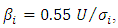
  being the surface friction velocity and is the depth of the neutral PBL. The dimensionless dissipation rate is defined as
 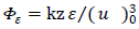 where
where  is the mean turbulent kinetic energy dissipation per unit time per unit mass of fluid, and its magnitude depends only on quantities that characterize the energy-containing eddies. The above
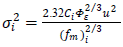
  values are derived from the turbulence isotropy in the inertial subrange of the energy spectrum.The analytical integration of Eq. (2) over the whole frequency domain leads to the Eulerian turbulent velocity variance [1, 7]
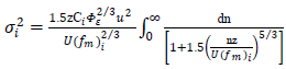 | (3) |
 | (4) |
 | (5) |
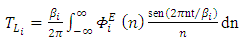
 yields as ref. [7]
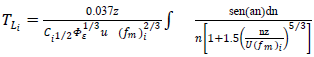 | (6) |
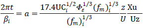 where a time to space transposition is applied to the time dependency in Eq. (1) to yield a spatially dependent
  with
with 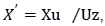 being a dimensionless distance defined by the ratio of travel time
  to the shear turbulent timescale
  .Defining
  where
where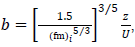 Eq. (6) can be written as
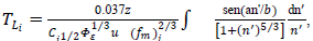 | (7) |
 | (8) |
 must be inferred from field observations at a shear-dominated PBL. For the neutral case, the spectral peak frequency
  describes the spatial and temporal characteristic scales of the energy-containing eddies, and can be expressed as Refs. [5, 14-16]:
 | (9) |
 is the spectral peak frequency at the surfa-ce,
  is the Coriolis parameter, and
 and
and  [8]. In the present study, the values of
  and the spectral peak frequencies
  have been measured during a meteorological phenomenon known as north wind flow (NWF), which occurs in a regional scale at the center of Rio Grande do Sul state, in southern Brazil [14]. The atmospheric synoptic conditions associated to the NWF cases are characterized by intense mean wind speeds, so the large vertical wind shear was produced predominantly by mechanical turbulence.Therefore, one of the main peculiarities of the present turbulent parameterization (values of
  and
and  obtained from the NWF cases) is that it regards the turbulent dispersion in neutral situations. For a more detailed discussion on the turbulence measurements taken during NWF events we suggest the paper by Arbage et al. [14]. The observations indicate that the mean values of
  are [14]:
 and
and 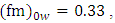 which are in fair agreement with those obtained at the classic Kansas and Minnesota micrometeorological experiments [15]. At neutral stability atmospheric condition one expects that
  approaches unity, due to the balance between shear production and viscous turbulence dissipation in the absence of any buoyant production and transport. Thus the value of
  obtained from the inertial subrange of the vertical velocity spectra is in good agreement with Kansas results [15, 16] and with theoretical predictions [14, 16, 17]. At this point it is important to note that the role of the NWF data in the present analysis is to provide the values of
  and
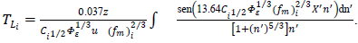
and  for Eqs. (4), (8) and (9). For large winds, such as those occurring during NWF cases, a neutral stability state in the PBL can be considered. Thus, for strong winds, mechanical turbulent forcing balances and dominates the thermal effects and consequently the real PBL can be assumed in a neutral condition.The Lagrangian decorrelation timescales for the velocity components u, v and w can be derived from Eq. (8) by assuming empirical values for the NWF data. To proceed, the Lagrangian decorrelation timescales can be obtained from Eqs. (8) and (9) as a function of both the downwind distance X′ and of the height z using Ci ,
  and
and  and [14, 18, 19]:
 | (10) |
 | (11) |
 | (12) |
 | (13) |
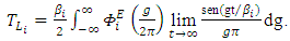
2.1. Asymptotic Behaviour of Eq. (1)
- The asymptotic behaviour of Eq. (1) can be derived considering the fact that
 where
where  is an Eulerian even two-sided spectrum normalized by the Eulerian velocity variance
  by [25].Substituting
 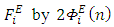 in Eq. (1) yields
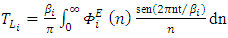 | (14) |
 | (15) |
 Eq. (15) can be written as
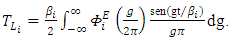 | (16) |
 | (17) |
 in Eq. (17) we get
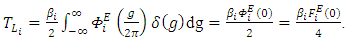 | (18) |
 with an asymptotic behavior can be derived from Eqs. (18) and (5) according to [1]:
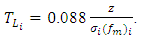 | (19) |
 and
and  can be derived from Eq. (19) assuming empirical values for the NWF data.
 | (20) |
 | (21) |
 | (22) |
3. Model Evaluation
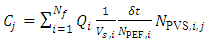
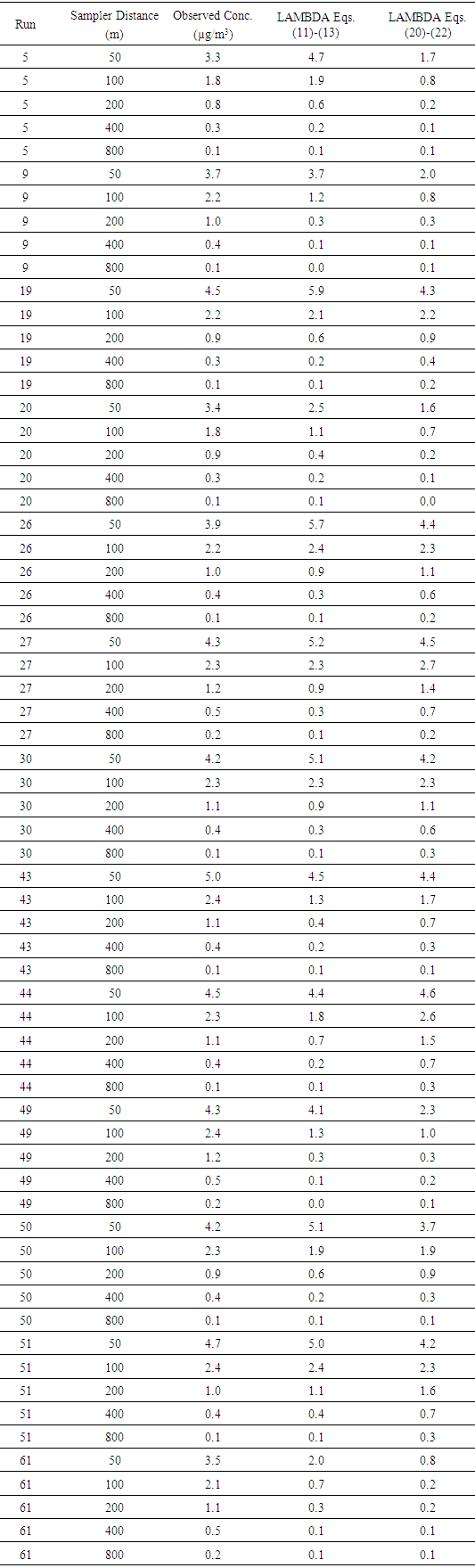
- In this section, the Lagrangian decorrelation timescales derived in Section 2 (Eqs. (11-13) and (20-22)) are introduced in the LAMBDA model, with the purpose of evaluating the performance of the solution in reproducing experimentally observed ground level concentrations. To this end, SO2 tracer data concentrations from the Prairie Grass dispersion experiment carried in O’Neill, Nebraska, in 1956, will be considered in that experimental campaign, contaminants (SO2) were emitted without buoyancy from a 0.46 m height and sampled at a height of 1.5 m at five downwind distances (50, 100, 200, 400, 800 m) [31]. The Prairie Grass site was flat with a 0.6 cm roughness length. From the Prairie Grass runs, thirteen cases in which the mean wind speed was greater than 6.0 ms−1 with values of
 were selected. Table 1 provides the values of the micrometeorological parameters for the selected Prairie Grass runs. The values of
  and
and  expressed in Table 1, are characteristic of a neutral PBL [32]. Therefore, the turbulent parameters
  , obtained for a neutral PBL from NWF data (strong wind velocity cases), can be used in Eqs. (11-13) and (20-22) to simulate the measured concentrations for these selected neutral Prairie Grass experiments. The wind speed profile used in the simulations follows a power law, being expressed as Ref. [33].
4. Description of the LAMBDA model
- LAMBDA is based on a three-dimensional form of the Langevin equation for the random velocity according to Thomson [34]. It is assumed in Thomson [34] that the evolution of the marked fluid particle displacement and velocity
 is a Markov process (past and future are statistically independent when the present is known). The velocity and the displacement of each particle are given by the following equations:
 | (23) |
 | (24) |
 is the displacement vector,
  the mean wind velocity vector,
  the Lagrangian velocity vector (velocity of a fluid particle associated to the turbulent velocity fluctuation [35]),
  is a deterministic term,
  is a stochastic term and the quantity
  are the increments of the Wiener process, an aleatory increment in the Gaussian distribution with zero mean and
  variance. From the descriptions of
  and
and  the numerical integration of equation (23), yields the turbulent velocity and the result complements equation (24), for the establishment of the particle position due to the combined effects of mean wind and turbulent velocity. These equations define the successive particle positions in the domain simulation under the influence of the mean wind and turbulent velocity.The determination of the
  coefficient implies to impose the well-mixed condition, so that the trajectory of the particles should prevail mixed in the flow. The well-mixed criteria is satisfied by the probably density function (PDF) of the Eulerian velocity,
  when the Fokker-Planck equation satisfies equations (23) and (24). The stationary Fokker-Planck equation is given by
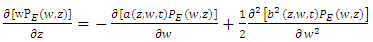
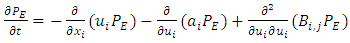 | (25) |
 and
and  are the Eulerian probability density function of the turbulent velocity. Equation (25) give the relation between the function
  and the Eulerian statistics characteristics of the turbulent flow, represented by the probably distribution
  Thus the terms in the right hand side of the Fokker-Planck equation represent the advection, the convection and the turbulent diffusion, respectively. The deterministic coefficient
  is obtained from
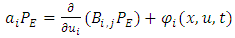 | (26) |
 | (27) |
 The deterministic coefficient
  is obtained from equation (26) as
 | (28) |
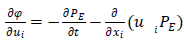
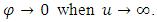
 In equation (26), the first term represents the fading memory and the second term a drift, which is a spatial function of the velocity gradient. In equation (26) one needs to determine the function
 . According to [34] a particular solution is the Gaussian velocity distribution. Therefore, Thomson used equation (27) to obtain the following expression for
 | (29) |
 is determined by comparing the structure function of the Lagrangian velocity, derived from Equation (23).
 | (30) |
 [22].
[22].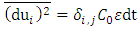 | (31) |
 are related to the constants
  by
by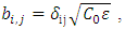 | (32) |
 is the Kronecker delta,
  is the Kolmogorov constant and
  is dissipation rate of turbulent kinetic energy mentioned before, and this constant of the structure function is a crucial quantity for Lagrangean stochastic particle modeling. The operation
  also can be represented as a function of the variance of velocity fluctuations
  and a Lagrangean decorrelation timescale
  [28, 29]:
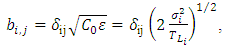 | (33) |
 and decorrelation timescales
  or the turbulent kinetic energy dissipation rate
  and the Kolmogorov constant
  [21]. In the representation of vertical speed, in a stochastic Lagrangian particle model, an asymmetry must also be considered. Especially in the presence of physical phenomena known as updrafts and downdrafts. These phenomena occur when sun radiation heats the ground and transfer of heat occurs from the ground to the air. Then an asymmetry exists, because updrafts have higher speeds and occupy a smaller crossing area. Differently, downdrafts have lower speeds and occupy a larger area. Normally, this kind of characteristics is more applicable to an unstable planetary boundary layer. However, vertical asymmetric motions can exist and influence the particle movements [10]. Therefore an asymmetric PDF is required and has been proposed by Luhar and Britter [36] and Weil [38], introduced by Baerentsen and Berkowicz [37]. The construction of the PDF is performed by a linear combination of two Gaussian distributions.The Langevin model for the vertical coordinate is written as follows:
 | (34) |
 | (35) |
 | (36) |
 are the same for the horizontal Langevin equation. According to [34], a simplification may be applied to the coefficient as
  Then the Langevin equation can be rewritten as:
 | (37) |
 | (38) |
 resulting in the following equations,
 | (39) |
 | (40) |
 depend on the Eulerian PDF
  an is obtained from (38). Thomson [34] states that the Fokker-Planck equation can be divided in two expressions that satisfy the well-mixed condition:
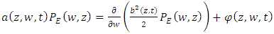 | (41) |
 | (42) |
 In this latter case, two different approaches can be adopted in order to calculate the Fokker-Planck equation: a bi-Gaussian one, truncated to the third order, and a Gram-Charlier one, truncated to the third or to the fourth order [39, 9]. The bi-Gaussian PDF is given by the linear combination of two Gaussians [37] and the Gram-Charlier PDF is a particular type of expansion that uses orthonormal functions in the form of Hermite polynomials. In this work was used the Gram-Charlier truncated to the third order. The FDP Gram-Charlier, truncated to the fourth order is given in reference [40].
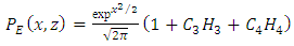 | (43) |
 are Hermite polynomials and
  and
and  are the coefficients of the Hermite polynomials.
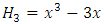 | (44) |
 | (45) |
 | (46) |
 | (47) |
 are the moments of
  and
and  In a Gaussian turbulence the equation (45) reduces to normal distribution
  equal to zero). Solving equations (41) and (42) where
  is given by (43) the following expression for
  can be found.
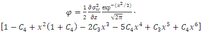 | (48) |
 [10].
[10].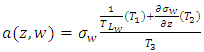 | (49) |
 | (50) |
 | (51) |
 | (52) |
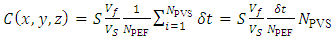
 In the LAMBDA model, the concentration field is determined from the trajectory of the particle in the flow. When the particle displacement in a turbulent flow has the stochastic behavior, the position of each particle in every time step is given by the larger probability to find this particle [41]. From the numerical point of view, the turbulent diffusion of pollutants in the planetary boundary layer is much more adequate from a Lagrangian reference frame, due to the simpler mathematical expressions [10]. The particles are emitted from the source position
  and the concentration is evaluated by a sensor position
  The domain is divided into sub-domain centered in
  , representing the sensor volume. The concentration is then estimated based on the time of stay of each particle in the sensor volume. The time resident in the sensor volume is evaluated counting the number of particles in the time interval
 | (53) |
 is the number of emitted particles in the source position in each time step
  is the number of particles in the sensor,
  is the sensor volume and
  is the volume source. The concentration in each sensor was calculated by the following expression:
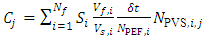 | (54) |
 is the number of particles emitted in the i-th source and
  is the number of particles emitted by the i-th source and detected in the j-th sensor. The emission intensity of i-th source is:
 | (55) |
 | (56) |
|
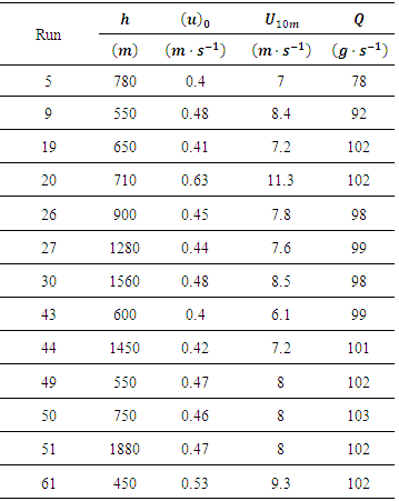
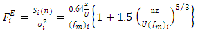
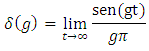
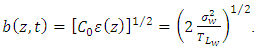
 | Figure 1. Scatter diagram of modeling results in comparison with observed ground-level concentration |
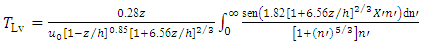
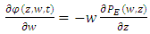
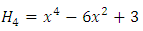
 for five different heights, as given by Eq. (12), is presented in Figure 2. Figure 3 shows the behavior of vertical profiles of
  as given by Eq. (12). Particularly, for Eq. (12) are plotted vertical profiles for three different distances from the source (x= 50, 100, 200, 400 and 800 m). Each profile represents a well behaved Lagrangian decorrelation timescale with a maximum varying height of the neutral boundary layer and with small values at z = 0 and z = h.
 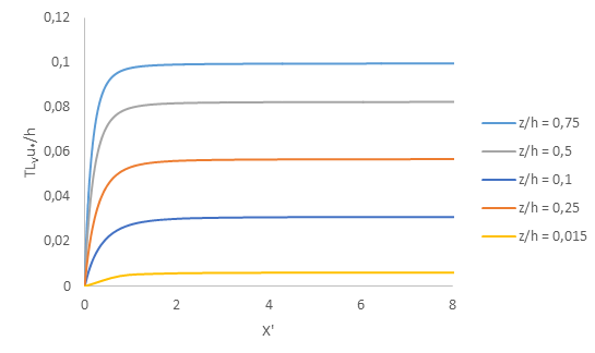 | Figure 2. The behaviour of the Lagragian decorrelation timescale TLy for five different heights z/h = 0.015, z/h= 0.25, z/h= 0.1, z/h= 0.5 and z/h= 0.75 as given by Eq. (12) and their asymptotic limit for far-source distances |
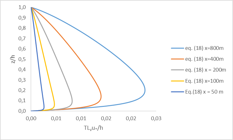 | Figure 3. The behaviour of the vertical profiles for the Lagrangian decorrelation timescales, depending on source distance for five different distances x= 50, 100, 200, 400 and 800m (Eq. (12) |
|
5. Conclusions
- A general development to obtain a new parameterization of decorrelation time scales that depend on source distance for a shear driven turbulent PBL has been proposed. The approach is based on the Eulerian velocity spectra and a formulation of the evolution of the Lagrangian decorrelation timescales. The derived decorrelation time scales are valid in the near, intermediate, and far ranges from a continuous point source. Employing turbulent parameters that were measured during an intense wind phenomenon known as north wind flow [14] the current model provides an integral formulation for the vertical, crosswind and along wind decorrelation time scales that depends on the distance from the source for inhomogeneous turbulence in a neutral PBL. Such decorrelation time scales, calculated from a complex integral, have been compared to a simpler asymptotic formulation. Therefore, the asymptotic and the memory flow formulation was introduced in a stochastic air pollution model, and compared to concentration data from the classical Prairie Grass experiments. The Prairie Grass selected runs employed in this work were accomplished in a neutral PBL. Therefore, the relevant role of the north wind measurements in this study is those to supply magnitudes of
 and
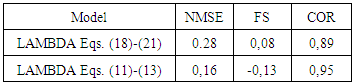
and  for a neutral PBL. These values were used to obtain Eqs. (11-13) and (20-22). This explains the importance of the north wind data in the present analysis and their connection with the Prairie Grass neutral experimental runs.The performance of the dispersion model using the asymptotic formulation evaluated by specific statistical indices shows a good degree of agreement between the asymptotic and integral formulations. Furthermore, the integral formulations with the memory effect that depends on the distance from the source are much more correlated to the Prairie Grass observations. The scatter diagram (Fig. 1) and the statistical indices (Table 3) show a good agreement between the modeled results and the experimental ones. Specifically, the statistical indices COR and NMSE allow to conclude that the results obtained with the decorrelation time scales depends on the source distance (Eqs. (11-13)) are better than those reached using an asymptotic decorrelation time scales (Eq. (20-22)), valid only for the far range from a continuous point source. Therefore, the current analysis suggests that the inclusion of the memory effect in the decorrelation time scales, improves the description of the turbulent transport of atmospheric contaminants released from a low continuous point source.
|
ACKNOWLEDGEMENTS
- The authors thank CNPq (Conselho Nacional de Desenvolvimento Científico e Tecnológico) for the partial financial support of this work.