Juliana Schramm, Franco C. Degrazia, Marco T. M. B. Vilhena, Bardo E. Bodmann
Department of Mechanical Engineering, Federal University of Rio Grande do Sul, Brazil
Correspondence to: Juliana Schramm, Department of Mechanical Engineering, Federal University of Rio Grande do Sul, Brazil.
| Email: |  |
Copyright © 2016 Scientific & Academic Publishing. All Rights Reserved.
This work is licensed under the Creative Commons Attribution International License (CC BY).
http://creativecommons.org/licenses/by/4.0/

Abstract
This study aims to compare the wind and concentration field generated by a coupling of WRF/CALMET model and CALMET/CALPUFF with no introduction of any gridded wind field. The domain was located at the city of Linhares, southeast region of Brazil, with a 15×15 grid cells and 1 km resolution. The chosen modelling period was April 1st, 2011, with the length of 90 h. The pollutants simulated by CALPUFF were NO2 and SO2. The final results of dispersion and concentration peak were compared against environmental legislation of 1 h average for NO2 and 24 h average for SO2. The first simulation, using WRF/CALMET model, shows plausible results. The second mode, CALMET/CALPUFF, generated a wind field with questionable results, which probably compromised the dispersion simulation. Both model results are within environmental legislation.
Keywords:
WRF, CALPUFF, Dispersion, Model, Brazil
Cite this paper: Juliana Schramm, Franco C. Degrazia, Marco T. M. B. Vilhena, Bardo E. Bodmann, Comparison of CALMET and WRF/CALMET Coupling for Dispersion of NO2 and SO2 Using CALPUFF Modelling System, American Journal of Environmental Engineering, Vol. 6 No. 4A, 2016, pp. 50-55. doi: 10.5923/s.ajee.201601.08.
1. Introduction
The air quality and the concentration of pollutants in the atmosphere are one of the many concerns about people’s health. According to the 1st Diagnosis of Air Quality Monitoring Network in Brazil [1], the country faces a lack of monitoring sites and atmospheric pollution measurements when compared with air quality standards, national and international. There are possibilities to evaluate the concentration of pollutants of a region with no monitoring sites by using dispersion models such as AERMOD, CALPUFF, ISC3 and others. This study is focused on a region of southeast of Brazil where a power plant is located near the city of Linhares.The power plant of Linhares uses natural gas as fuel, which releases sulphur dioxide, nitrogen oxides, particulate matter, carbon oxides and other hydrocarbons in smaller quantities when combustion occurs. The major fraction emitted in burning of the natural gas is nitrogen oxides, formed by heating the air around the combustion point [2]. The Environment Ministry of Brazil considers these species atmospheric pollutants and therefore a study of its dispersions is required to suit the environmental legislation.
1.1. Background
CALPUFF is one of the models that is recommended by the United States Environmental Protection Agency (USEPA) [3]. It is a non-steady-state Lagrangian Gaussian puff model and includes three components: CALMET, CALPUFF and CALPOST. CALMET is a meteorological model that contains an option to allow the introduction of gridded wind fields generated by MM4/MM5 and WRF models as input fields. That option may better represent regional flows and certain aspects of sea breeze circulations and slope/valley circulations [4].Several studies have been made in order to evaluate the performance of coupling MM5 and WRF with the CALMET model. Using MM5’s output as an initial guess field in CALMET, Cui et. al [5] noted that the model can correctly capture the shape and direction of tracer experiments, but hourly resolution of meteorological data may be too coarse to predict the short-range dispersion and may induce some errors. A similar experiment was done by Gopalaswami et al. [6], who compared CALMET/MM5 results with data from a meteorological station. The authors concluded that utilizing the coarsest prognostic meteorological model output into a diagnostic model provides a feasible option for generating meteorological inputs for risk analysis. Chandrasekar et al. [7] investigated the usefulness of coupling MM5 with CALMET by comparing the results of simulation of MM5/CALMET and CALMET only. The results indicate that the predictions in the first mode are much closer to observations as compared to the second mode. In 2014, Lee et al. [8] used WRF/CALPUFF modelling tools to evaluate the concentration of PM10 and SO2 emitted from industrial complexes in Korea. The results obtained by meteorological and concentration field simulated showed a good agreement with the observed data. This background shows that the coupling of meteorological models such as MM5 and WRF with CALMET produces results that are closer to observational data. In this study we used the coupling of WRF and CALMET modelling systems to compare the results of meteorological field and dispersion of the pollutants sulphur and nitrogen dioxides with the CALMET/CALPUFF model. To check air quality although with lacking measured data we compared the data obtained by the two simulations against restrictions from environmental legislation.
2. Methodology
2.1. Area of Study
Linhares is a city in the state of Espírito Santo, southeast region of Brazil. In this year the total area and population of the city are 3 504.137 km² and 163 662 people, respectively, according to Brazilian Institute of Geography and Statistics (IBGE) [9]. The area of this study covers a power plant with height 5-8 m above sea and is located 4 km from the coast, the topography of the area is considered flat. The climate in this region is predominantly tropical, the annual average temperature is above 20°C and the annual wind speed is about 3-3.5 m/s at 10 m, according to the National Meteorology Institute (INMET) [10]. The knowledge of the meteorological and geographical conditions is important since it has a significant impact on the dispersion and concentration of pollutants [11].
2.2. Environmental Legislation
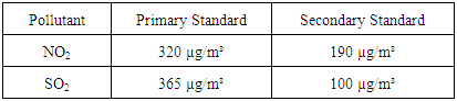
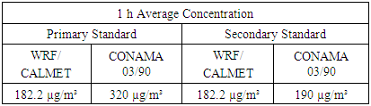
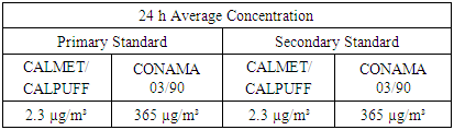
The current legislation of Brazil about air quality was created by the National Environment Council (CONAMA) and is called Resolution No. 03 of 1990 – or CONAMA 03/90. That resolution sets two standards of air quality: the Primary consists in the concentration of pollutants which, if exceeded, can affect the population’s health; and the Secondary if the concentration of pollutants is below, provides the least adverse effect on the environment in general. The standard concentration for NO2 are measured in 1 h average and for SO2 in 24 h average, the values are shown in Table 1 [12]. The annual concentrations are not used in this study, since the simulation was made in a period of time less than one year.Table 1. Primary and Secondary Standard for NO2 and SO2, by CONAMA 03/90
 |
| |
|
2.3. WRF/CALMET Model
In order to develop the wind field and visualize the dispersion of atmospheric pollution emitted by the sources, the CALPUFF model was used. The CALPUFF Modelling System was developed by Sigma Research Corporation and the version used in this study was approved by USEPA. The software requires a large set of pre-processing programs designed to interface the model with standard, routinely-available meteorological and geophysical datasets [4].The pre-processors used were TERREL, CTGPROC and MAKEGEO. The model domain was a 15 km by 15 km area, with a grid resolution of 1 km. The starting date is April 1st, 2011 and the length of run 90 h. TERREL is a terrain pre-processor that uses a topographical data, which was obtained from WebGIS website [13], and produces a gridded terrain file for the MAKEGEO. CTGPROC reads a land use and land cover data, obtained from USGS website [14] in this work, and determines fractional land use for each grid cell. The outputs of TERREL and CTGPROC were used as an input at MAKEGEO that creates a geophysical data file.To simulate the meteorological model CALMET was used that computes hourly gridded wind field and micrometeorological variables. As inputs were used the output of MAKEGEO pre-processor and the output of WRF, which act as initial and boundary conditions of the meteorological variables. CALMET then uses the WRF’s output to generate a meteorological field downscaled and establish all the micrometeorological variables needed for dispersion simulation [15]. To visualize the results of this simulation the use of the post-processor PRTMET is of need.CALPUFF uses the meteorological field created by CALMET to simulate the transport and dispersion of puffs of material emitted from modelled sources. The power plant studied on this paper has 24 point sources and data from each source has been included into the model, such as stack height, base elevation, stack diameter, exit velocity and temperature, etc. The post-processor CALPOST was used to visualise the model results.
2.4. CALMET/CALPUFF Model
In this second simulation, the output of WRF model was not used as CALMET input. The pre-processors TERREL, CTGPROC and MAKEGEO have been also used. To generate a meteorological model two other pre-processors were required: SMERGE and READ62.SMERGE processes hourly surface observation data from stations and reformats this data into a single file to be used in CALMET. The pre-processor reads files containing surface data in CD144, SAMSON or HUSWO formats. In this study, SAMSON format was used with observational data obtained from Vitória’s airport station, available at CPTEC [16] and INMET [17] websites.READ62 extracts and processes upper air wind and temperature data, obtained from NOAA website [18], into a form required by CALMET model. The output file produced by READ62 contains the pressure, elevation, temperature, wind speed, and wind direction at each sounding level.Using the outputs of these pre-processors, the CALMET and CALPUFF models were simulated at the same conditions and parameters of the first simulation, in order to compare both results.
3. Results and Discussion
PRTMET and CALPOST post-processors are needed to visualize the results of the meteorological model and the dispersion of pollutants, respectively.
3.1. WRF/CALMET Results
The results of coupling WRF model and CALPUFF System are shown in this section. All results show x and y axes as Cartesian coordinates, in km, of the studied site, where the power plant is located.The results of a meteorological wind field produced by WRF/CALMET simulation are shown in Figure 1. The vectors indicate the wind speed and direction and the size of the vector is proportional to wind speed. The colour scale on the side shows the average wind speed at 90 h simulation, measured in m/s.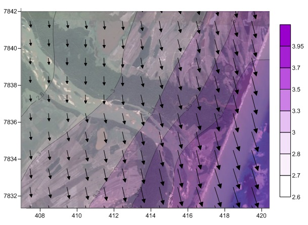 | Figure 1. Average direction and wind speed at 90 h simulation using WRF/CALMET model (m/s) |
In order to have a better representation of the wind speed near the power plant, a coordinate located close to the plant (415.453 km of latitude and 7839.483 km of longitude) was chosen to analyse the variation of wind speed versus simulation time. This representation is showed in Figure 2.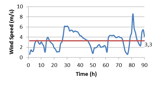 | Figure 2. Wind Speed versus Time using WRF/CALMET model |
The results presented by Figure 1 shows an average wind direction north-northwest and wind speed in the range from 2.6 to 3.95 m/s at 90 h simulation. The highest wind speed value is located near the ocean and decreases gradually as it advances toward the mainland.Figure 2 shows that near the power plant the average wind speed is about 3.3 m/s and varies from 1 m/s to 8 m/s. According to data from the meteorological station at Vitoria’s Airport the average wind speed (obtained for the same time period used on WRF/CALMET) was 2.3 m/s, as shown in Figure 3. This difference of average wind field exists due to two possible reasons: errors in the simulation and the distance of 131 km from the cities Vitoria and Linhares.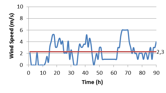 | Figure 3. Wind Speed versus Time, data from Vitoria’s Airport |
Figure 4 shows the dispersion of NO2 with the colour scale representing the concentration measured in µg/m³ at 90 h simulation.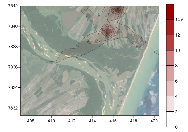 | Figure 4. Average NO2 concentration at 90 h simulation using WRF/CALMET model (µg/m³) |
Figure 4 shows that the NO2 concentration reaches the maximum value of 14.5 µg/m³. The concentration peak for 1h average is 182.2 µg/m³, according to CALPOST results. Both 90 h and 1 h average reach the concentration peak at coordinates 415.453 km and 7839.483 km. Table 2 shows the comparison of environmental legislation, CONAMA 03/90, and results of WRF/CALMET simulation.Table 2. Comparison of CONAMA 03/90 and WRF/CALMET Simulation for NO2
 |
| |
|
The results obtained for 1 h average are within environmental legislation, primary and secondary standards, as shown in Table 2.Figure 5 shows the dispersion of SO2 for 90 h simulation.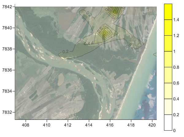 | Figure 5. Average SO2 concentration at 90 h simulation using WRF/CALMET model (µg/m³) |
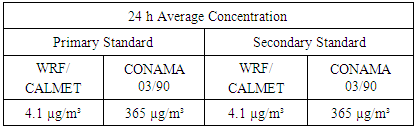
The maximum concentration of SO2 is 1.4 µg/m³ at 90 h simulation as shown in Figure 5, in the same coordinate system as NO2. For 24 h average the concentration peak is 4.1 µg/m³, located at 416.453 km and 7839.483 km coordinates. The concentration values for SO2 are considerably lower than those obtained for NO2 since nitrogen oxides are the main pollutant emitted from natural gas combustion [2]. Table 3 shows the comparison of CONAMA 03/90 and simulation.Table 3. Comparison of CONAMA 03/90 and WRF/CALMET Simulation for SO2
 |
| |
|
Table 3 shows that the results for SO2 are below both primary and secondary standards.
3.2. CALMET/CALPUFF Results
The same analysis of the first simulation was made in the CALMET/CALPUFF. Figure 6 represents the average wind speed and direction and Figure 7 shows the wind speed versus simulation time, using the same coordinates of WRF/CALMET.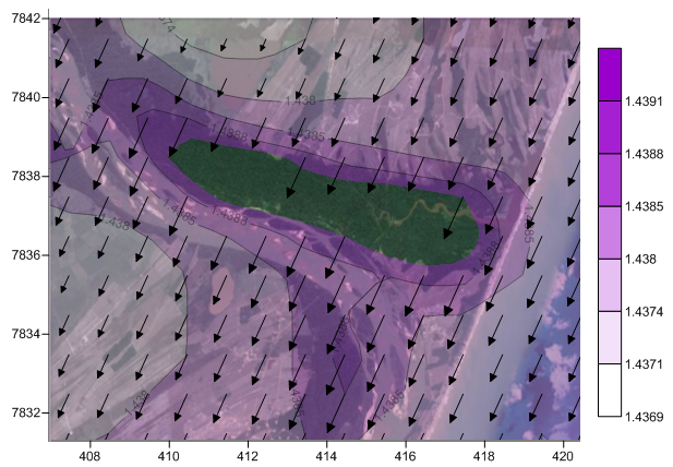 | Figure 6. Average direction and wind speed at 90 h simulation using CALMET/CALPUFF model (m/s) |
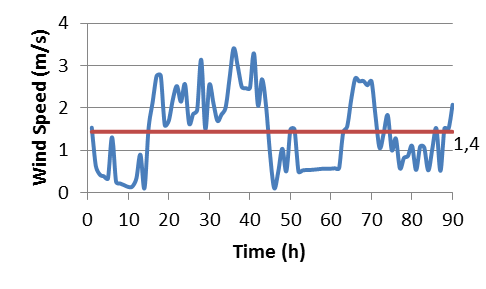 | Figure 7. Wind Speed versus Time using CALMET/CALPUFF model |
The results for wind field presented in Figure 6 shows an average wind direction north-northeast. The average wind speed varies on the thousandth decimal place only, and remains practically constant at 1.4 m/s throughout the studied grid.Figure 6 shows a lack of results in the middle of the grid. That occurs probably because there’s not enough public data from meteorological stations, a fact that was already published by the 1st Diagnosis of Air Quality Monitoring Network in Brazil.Figure 7 shows that at the coordinate near the power plant the average wind speed is also 1.4 m/s. This value is below 2.3 m/s, average wind speed of Vitoria’s Airport showed at Figure 3.Figure 8 shows the average concentration of NO2 obtained by CALMET/CALPUFF simulation.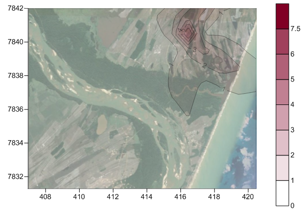 | Figure 8. Average NO2 concentration at 90 h simulation using CALMET/CALPUFF model (µg/m³) |
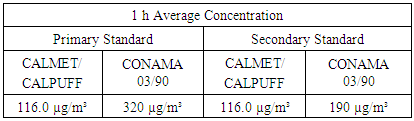
Figure 8 shows that the maximum value of concentration for NO2 is 7.5 µg/m³ at 90 h simulation. For 1 h average 116.0 µg/m³ is the concentration peak obtained by CALPOST results. Both peaks are located at the same coordinates, 416.453 km and 7840.483 km. Table 4 shows the comparison of the 1 h average simulation results and CONAMA 03/90.Table 4. Comparison of CONAMA 03/90 and CALMET/CALPUFF Simulation for NO2
 |
| |
|
The results of CALMET/CALPUFF are below primary and secondary standards of CONAMA 03/90, as shown in Table 4.Figure 9 shows the 90 h dispersion results for SO2.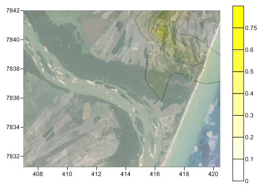 | Figure 9. Average SO2 concentration at 90 h simulation using CALMET/CALPUFF model (µg/m³) |
Figure 9 shows that 0.75 µg/m³ is the maximum value at 90h simulation and for 24 h average is 2.3 µg/m³. The coordinates where the peaks are located are the same as NO2. Table 5 shows the comparison of results with legislation.Table 5. Comparison of CONAMA 03/90 and WRF/CALMET Simulation for SO2
 |
| |
|
The results for 24 h average of SO2 are also within environmental legislation, as shown in Table 4.
4. Conclusions
This paper aims to evaluate the dispersion of the pollutants nitrogen and sulphur dioxides and the difference between a simulation with WRF as an input and a simulation without any input of wind field models. The period chosen for this study starts at April 1st of 2011 and has the length of 90 h.Results of WRF/CALMET model show a north-northwest wind with speed of 2.6 to 3.95 m/s at 90 h simulation, the results of average wind speed near the power plant is above the one obtained by data from Vitoria Airport. The maximum concentration values for NO2 and SO2 were 14.5 and 1.4 µg/m³, respectively. The 1 h and 24 h average results are within environmental legislation, CONAMA 03/90. The behaviour of wind direction and dispersion can be considered realistic.CALMET/CALPUFF simulation shows a wind field with lack of results into the studied grid. The wind speed found was practically constant at 1.4 m/s, that is smaller than Vitoria’s Airport average wind speed. The results for NO2 and SO2 concentrations are around 1.6 times smaller than the first simulation and therefore are within air quality standards set by CONAMA 03/90. Due to the lack of results on the gridded wind field the dispersion model obtained by this simulation can be considered quastionable, since the wind field generated has an important impact on dispersion results.The authors are aware of lack of validation of the results obtained by the absence of experimental data, but it is possible to propose suitable sample sites for future verification in the location of found concentration peaks. The continuation of this work is focused on numerical validation of the model using concentration data of measurements in the plant and the model evaluation for a period of one year to obtain results with greater reliability limits.
ACKNOWLEDGEMENTs
The authors acknowledge CNPq for financial support. Some of the authors thank Linhares Geração SA, Tevisa and ANEEL P&D for financial support.
References
| [1] | Energy and Environment Institute, 2014. 1st Diagnosis of Air Quality Monitoring Network in Brazil. |
| [2] | S. Mokhatab, W. A. Poe, J. G. Speight, 2006, “Handbook of Natural Gas Transmission and Processing”, Elsevier Inc., Burlington. |
| [3] | USEPA, 2016. Preferred/Recommended Models [Online]. Available: www3.epa.gov/scram001/dispersion_prefrec.htm. |
| [4] | J. S. Scire, D. G. Strimaitis, R. J. Yamartino, 2000, “A User’s Guide for the CALPUFF Dispersion Model (Version 5)”, Earth Tech Inc., Concord. |
| [5] | H. Cui, R. Yao, X. Xu, C. Xin, J, Yang, 2011, “A tracer experiment study to evaluate the CALPUFF real time application in a near-field complex terrain setting”, Atmospheric Environment 45, 7525-7532. |
| [6] | N. Gopalaswami, K. Kakosimos, L. Vèchot, T. Olewski, M. S. Mannan, 2015, “Analysis of meteorological parameters for dense gas dispersion using mesoscales models”, Journal of Loss Prevention in the Process Industries 35, 145-146. |
| [7] | A. Chandrasekar, C. R. Philbrick, R. Clark, B. Doddridge, P. Georgopoulos, 2003, “Evaluating the performance of a computationally efficient MM5/CALMET system for developing wind field inputs to air quality models”, Atmospheric Environment 37, 3267-3276. |
| [8] | H. Lee; J. Yoo; M. Kang; J. Jung; K. Oh, 2014, “Evaluation of concentrations and souce contribution of PM10 and SO2 emitted from industrial complexes in Ulsan, Korea: Interfacing of the WRF-CALPUFF modeling tools”, Atmospheric Pollution Research 5, 664-676. |
| [9] | IBGE, 2015, Database – Cities - ES [Online]. Available: http://cidades.ibge.gov.br/xtras/perfil.php?codmun=320320. |
| [10] | INMET – Normal Climatological – Average Temperature Compensated 1961-1990 [Online]. Available: http://www.inmet.gov.br/portal/index.php?r=clima/normaisClimatologicas. |
| [11] | S. A. Abdul-Wahab, K. Chan, A. Elkamel, L. Ahmadi, 2014, “Effects of meteorological conditions on the concentration and dispersion of an accidental release of H2S in Canada”, Atmospheric Environment 82, 316-326. |
| [12] | CONAMA - Resolution No. 03 of 1990, establishing the primary and secondary standards of air quality and criteria for acute episodes of air pollution [Online]. Available: http://www.mma.gov.br/port/conama/res/res90/res0390.html |
| [13] | WebGIS – Geographic Information System Resource [Online].Available:http://dds.cr.usgs.gov/srtm/version2_1/SRTM3/South_America/. |
| [14] | USGS – United States Geological Survey [Online]. Available: http://edc2.usgs.gov/glcc/glcc_version1.ph. |
| [15] | J. Schramm, F. C. Degrazia, B. Bodmann, M. T. M. B. Vilhena, 2015, “Dispersão de poluentes de uma usina termelétrica localizada em Linhares, utilizando o modelo CALPUFF”, IX Brazilian Workshop Micrometeorology Proceedings. |
| [16] | CPTEC – Observational Data – Download – Metar [Online]. Available:http://bancodedados.cptec.inpe.br/downloadBDM/. |
| [17] | INMET – Meteorological Database for Education and Research [Online]. Available: http://www.inmet.gov.br/portal/index.php?r=bdmep/bdmep. |
| [18] | NOAA – ESRL Radiosonde Database [Online]. Available: http://esrl.noaa.gov/raobs/. |

 Abstract
 Reference
 Full-Text PDF
 Full-text HTML