1. Introduction

About one hour before sunset over land, the surface heat flux becomes negative and, consequently, a stable boundary-layer (SBL) develops near the ground [12, 17]. Above this SBL, in the residual layer (RL), the convective eddies start to lose their strength and the convective boundary-layer (CBL) begins to decay. The dispersion of pollutants by turbulent flows is of central importance in a number of environmental problems, but less attention has been paid to the dispersion in the RL, where the diffusion of pollutants occurs in conditions of decaying convective turbulence. The decay of energy-containing eddies in the CBL is the physical mechanism that can sustain the dispersion process in the RL.

Turbulence decay in the CBL has been studied by [12] using the dynamical equation for the energy density spectrum, by [5, 16, 17, 19, 20] employing LES models and by [9] employing a random displacement model. Experimental results has been reported by [1, 2, 10, 14, 15].

In this paper is investigated the turbulent dispersion process occurring during the sunset transition, focusing the characteristic patterns of the turbulent dispersion of pollutants released from a continuous point source in a diffusive PBL characterized by a decaying convective one. This analysis considers an analytical solution of the advection-diffusion equation, in which the turbulent effects are represented by eddy diffusivities for a SBL proposed by [11] and for a decaying turbulence in the CBL proposed by [11]. The use of these convective decaying eddy diffusivities in air quality models will generate realistic turbulent patterns associated to the sunset transition time. The simulation procedure is realized according methodology presented in [9], which used the random displacement equation to examine the dispersion process of contaminants emitted from low and tall sources during sunset period.

Thus, with these parameterizations (stable below and convective decaying turbulence aloft), the analytical Eulerian model can be used to evaluate the influence of the decaying convective eddies on the concentration field of pollutants released by elevated continuous point sources during the sunset transition time and the first hours of SBL development. The reason why adopting an analytical procedure instead of using the nowadays available computing power resides in the fact that once an analytical solution to a mathematical model is found one can claim that the problem has been solved. It is provided a closed form solution that may be tailored for numerical applications such as to reproduce the solution within a prescribed precision. As a consequence the error analysis reduces to model validation only, in comparison to numerical approaches where in general it is not straight forward to disentangle model errors from numerical ones [7].

2. Turbulence Parameterization

The aim of this section to exhibit and discuss the eddy diffusivities that have been employed in the analytical model to simulate the concentration field of contaminants by an elevated continuous point source during the sunset transition time. So, it is necessary parameterize the turbulent transport in a shear-dominated stable PBL and the decaying convective elevated turbulent dispersion.

2.1. Parameterization of the Stable PBL

The following relationships for longitudinal, lateral and vertical eddy diffusivities derived by [11], represent the turbulent diffusion in a shear-dominated stable PBL:

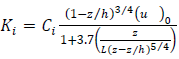(1)

in which and is the Obukhov length, is the surface layer friction velocity and h is the height of the stable layer. The magnitudes of the coefficients in the numerator of Eq. (1) show that the eddy vertical motion is strongly limited by the positive stratification.

2.2. Parameterization of the Residual Layer

A general method to derive eddy diffusivities in a decaying turbulence in the CBL has been proposed by [13]. The method is based on a model for the budget equation describing the energy density spectrum and the Taylor statistical diffusion theory. The turbulent field has been considered isotropic to calculate the longitudinal and lateral eddy diffusivities and non-isotropic to derive the vertical eddy diffusivity. The following relationships represent fits to the decaying convective eddy diffusivities obtained from the model proposed by [13]:

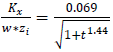(2a)

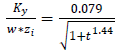(2b)

and

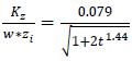(2c)

where is the height of the mixing layer, is the convective velocity scale and

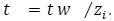
3. Eulerian Modelling

The Eulerian model considered here is represented by the advection-diffusion equation. We must recall that this equation is obtained combining the continuity equation ruled by the conservation law with the Fickian closure of turbulence. Indeed, we write the advection-diffusion equation in Cartesian geometry like [6]:

(3)

subject to the following boundary and initial conditions:

(3a)

(3b)

(3c)

(3d)

and by a source condition quoted as:

(3e)

where denotes the mean concentration of a passive contaminant, and are the cartesian components of the mean wind in the directions x (0 < x < L_x), y (0 < y < L_y) and z (0 < z < h) and and are the eddy diffusivities. Q is the emission rate, h the height of the atmospheric boundary layer, H_s the height of the source, L_x and L_y are the limits in the x and y-axis and far away from the source and represents the Dirac delta function. The source position is at and z = H_s.

Problem (3) is solved by the 3D-GILTT method [7, 8]. In the initial step it is expanded, without physical equivalence, the contaminant concentration in a series in terms of a set of orthogonal eigenfunctions. These eigenfunctions are the solution of a simpler but similar problem to the existing one. Replacing this expansion in the Eq. (3), the resulting problem reduces to a two-dimensional one already solved by the Laplace transform technique and GILTT method as shown in [15, 16]. For the simulations, the methodology presented by [15, 16] is considered. Here we assumed a Cartesian coordinate system in which the x direction coincides with the one of the predominant wind, the advection is much larger than the diffusion in the x-direction and the crosswind integration of the Eq. (3).

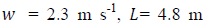
The micrometeorological parameters and 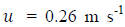[16] were considered for generating the eddy diffusivity profiles during the simulation. The simulations started at the moment of sunset when the surface heat flux progressively decreases and a stable boundary-layer develops near the ground. Profiles of eddy diffusivities suggested by [11] were informed to the stable boundary layer and derived by [13] (Eqs. 1-3) were informed to the residual layer. The evolution of the PBL height was calculated according to the expression [2], where h is given in meters and in hours. During the simulation, new profiles of eddy diffusivities and new values of SBL height were provided to the model in intervals according to Table 1.

Table 1. Simulation time       and SBL height according expression

4. Results

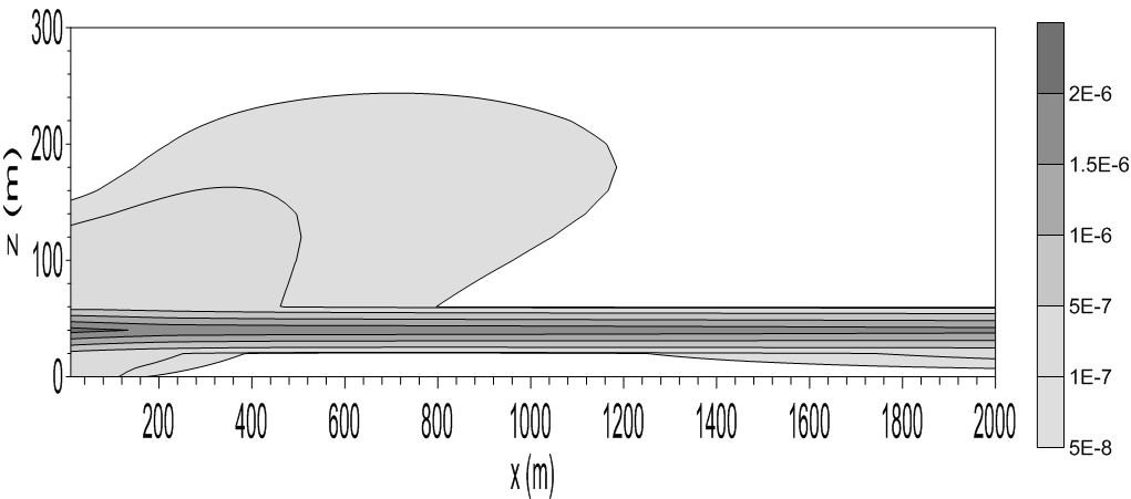
In this section is discussed the simulation results obtained with the Eulerian analytical model (Eq. 3) parameterized by the eddy diffusivities given by the Eqs. (1), (2a), (2b) and (2c). For the sunset transition period there will be analyzed the simulation of the cross-wind concentration field of contaminants released from a continuous point source at a height of 60m. The dispersion simulation is realized during the evolution time of the sunset transition according to Table 1.

Fig. 1 exhibits dispersion effects for the initial time of 900s and height of the stable layer of 35m. Analyzing the diffusion pattern associated to this figure it can be seen that the contaminants released from the source directly into the RL suffer a strong mixing action. This intense level of dispersion associated to the decaying turbulence in the RL is responsible for the entrance of contaminants to the interior of the SBL. It is possible to notice also that the contaminants go through in the interior of the SBL and reach the ground next to the point source. The dispersion effect of the decaying convective eddies in the RL over the plume of contaminant, pushes it down toward the top of the SBL and is captured by this new environment containing different diffusion properties. Then, the plume of contaminants disperses under the action of shear-dominated stable turbulence in the interior of the SBL. The stable turbulence from mechanical origin, is generated by the surface wind shear and consequently the energy-containing eddies in this layer are in the proximity to the surface. For a continuous stable turbulence, sustained by the mechanical forcing, the turbulent vertical velocity variance decreases with the height and this variance asymmetry (vertical inhomogeneous turbulence), induces an acceleration (drift velocity) that transports the contaminants in the direction to the surface where the wind shear turbulence diffusion action is dominant. This transport downward, associated to the wind shear turbulence above discussed, is particularly dominant in SBLs that present a small depth. In this thin initial SBL the effects of surface turbulence generation influence the major part of the SBL vertical extension.

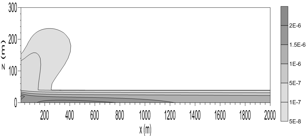Figure 1. Cross-wind concentration field (x-z plane). Source height of 60 m and stable boundary layer height of 35 m. Concentration in g m-2

Figs. 2 and 3 present the simulation results for the evolution times t = 1800s and 2700s, and heights of the stable layer of 50m and 60m, respectively. These figures exhibit the noticeable reduction of the concentration of contaminants in the surface due the SBL expansion and the loss of the diffusion capacity of the decaying convective energy-containing eddies. The loss of the diffusion capacity contributes to reduce the entrance of contaminants into the SBL and therefore to decrease the surface contaminant concentrations. The deepening of the SBL tends to engulf the RL region and covers the emission source, that reduces the dispersion process generated by the decaying convective eddies and the contaminants are emitted in an ambient where the diffusion is directed by mechanical turbulence. Figure 2 shows a configuration in which the maximum of concentration is increasingly inside the SBL. For the evolution time of 2700s, showed in Fig. 3, the height of the SBL reaches the height of the point source and consequently the contaminants are emitted into the SBL. For this source localization, the contaminants can travel long distances touch less the surface and, as result, the ground concentration is decreased as can be seen in figures 1-5. A quantity of contaminant, emitted during evolution times 900s and 1800s inside the RL, continues to experience the dispersion generated by the decaying convective eddies.

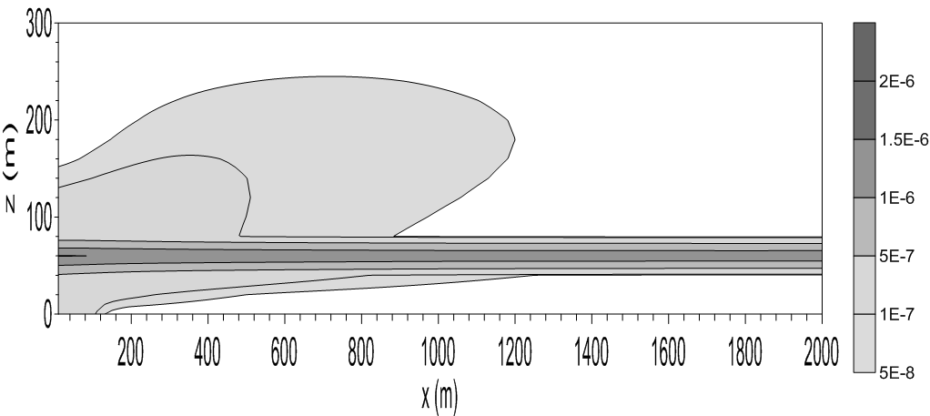
Figure 2. Cross-wind concentration field (x-z plane). Source height of 60 m and stable boundary layer height of 50 m. Concentration in g m-2

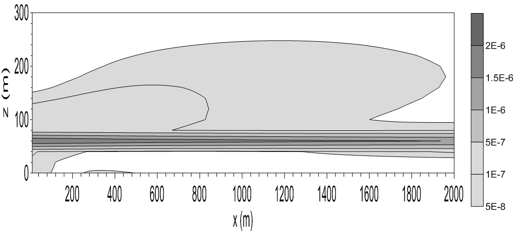
Figure 3. Cross-wind concentration field (x-z plane). Source height of 60 m and stable boundary layer height of 60 m. Concentration in g m-2

For the final phase of the sunset transition period the SBL height increases and supplants the contaminants point source height and hence the dispersion occurs in a stable boundary layer environment. In this stable turbulent field, characterized by small mechanical eddies, the low magnitude of the eddy diffusivities generates a very little spread in the vertical direction. This condition generate a fanning plume shape frequently observed in stable boundary layers, so that the plume acquires the shape of an angular fan, with a large spread in the horizontal and vary little spread, if any, in the vertical direction. This characteristic shape occurs typically at night in a very SBL with strong surface inversion and weak and variable winds [3]. This diffusion pattern is reproduced in Figs. 4 and 5, which show the crosswind concentration field for the final evolution times t= 3600s and t=4500s, respectively. The figures show that the plume travels for long distance and the maximum of the concentration remains in the same level of the emission source. The low magnitude of the eddy diffusivities generates a very little spread in the vertical direction and it avoids the arrival of contaminants in the surface. For these evolution times, the decaying convective eddies have still sufficiently energy for dispersing the contaminants emitted inside the RL when the SBL height was shorter than the source height. These results are similar to the ones obtained by [9] in a numerical approach, using a Lagrangian particle model.

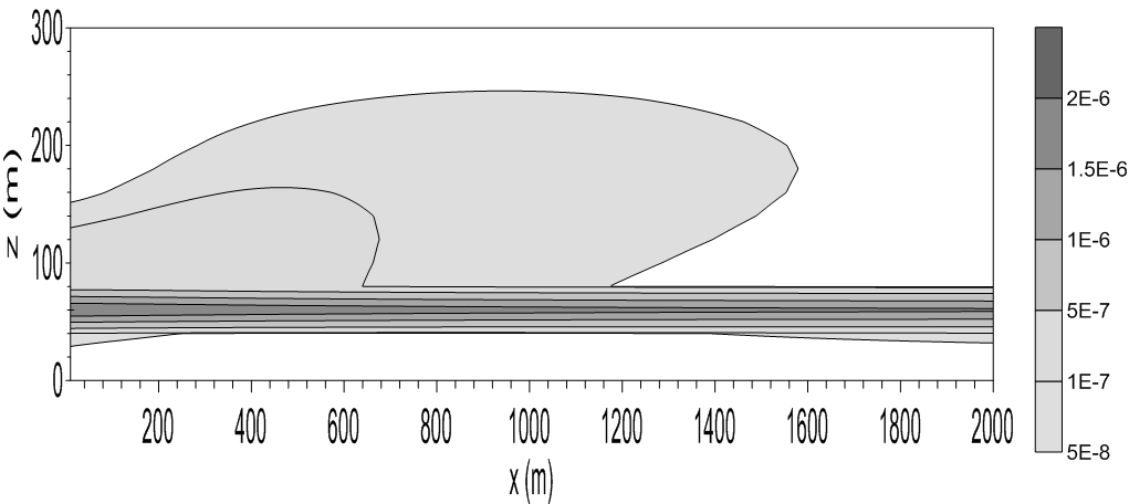
Figure 4. Cross-wind concentration field (x-z plane). Source height of 60 m and stable boundary layer height of 70 m. Concentration in g m-2

Figure 5. Cross-wind concentration field (x-z plane). Source height of 60 m and stable boundary layer height of 80 m. Concentration in g m-2

5. Conclusions

In this study an analytical description was employed to simulate the pollutants concentration released from continuous point source during the sunset transition period. The analysis applied the dispersion model parameterized by the stable and decaying convective eddy diffusivities, representing the turbulent mixing in the SBL and RL. The concentration simulations were calculated considering different times in the transition process through the sunset period. The simulations analyzed the crosswind concentration field of contaminants released from a continuous point source at a height of 60m.

The simulations showed that during the initial evolution times during the sunset transition, the turbulent diffusion generated by the decaying convective eddies in the RL caused an effective transference of contaminants to the interior of the SBL. During the initial stage, in which the SBL presents a small depth, the combination between residual convective and stable eddies acts efficiently to transport the pollutants in direction to the ground surface. Therefore, the present analysis showed that for this initial time, the combination between residual convective and stable eddies acts to transport the contaminants in direction to the ground, increasing the concentration at the surface.

For the final phase of the sunset transition period the SBL height reached the point source height and the dispersion occurred in a stable environment. This condition generated a fanning plume shape, which is characterized by a large spread in the horizontal and vary little spread in the vertical direction. The results showed that the plume traveled for long distance and the maximum of the concentration remains in the same level of the emission source. As a consequence of this lack of an effective turbulent mixing, acting over the whole vertical extension of the SBL, the contaminants do not arrive at the surface.

The results presented in this paper show similarity with ones reported in the literature, where the strong mixing action generated by the decaying convective energy-containing eddies in the RL causes an effective entrance of pollutants to the interior of the recently established SBL.

ACKNOWLEDGEMENTS

The authors acknowledge the financial support provided by CNPq (Conselho Nacional de Desenvolvimento Científico e Tecnológico), CAPES (Coordenação de Aperfeiçoamento de Pessoal de Nível Superior) and FAPERGS (Fundação de Amparo à Pesquisa do Estado do Rio Grande do Sul).