-
Paper Information
- Next Paper
- Previous Paper
- Paper Submission
-
Journal Information
- About This Journal
- Editorial Board
- Current Issue
- Archive
- Author Guidelines
- Contact Us
American Journal of Environmental Engineering
p-ISSN: 2166-4633 e-ISSN: 2166-465X
2016; 6(4A): 28-39
doi:10.5923/s.ajee.201601.05

On a Model for Pollutant Dispersion in the Atmosphere with Partially Reflective Boundary Conditions
 Abstract
 Reference
 Full-Text PDF
 Full-text HTML
Jaqueline Fischer Loeck1, Bardo E. J. Bodmann2, Marco T. M. B. Vilhena2
1Graduate Program in Mechanical Engineering, Federal University of Rio Grande do Sul, Porto Alegre, Brazil
2Federal University of Rio Grande do Sul, Porto Alegre, Brazil
Correspondence to: Jaqueline Fischer Loeck, Graduate Program in Mechanical Engineering, Federal University of Rio Grande do Sul, Porto Alegre, Brazil.
| Email: |  |
Copyright © 2016 Scientific & Academic Publishing. All Rights Reserved.
This work is licensed under the Creative Commons Attribution International License (CC BY).
http://creativecommons.org/licenses/by/4.0/

The present work is an attempt to simulate stochastic effects in a deterministic model for pollutant dispersion in the atmospheric boundary layer by the use of a probability weighted boundary condition. More specifically, the escape of pollutant substances across the boundary layer horizon on the one side and the surface boundary on the other side are modelled by probabilities to quantify the fraction of pollutant that returns into the boundary layer from above and the process of adsorption or deposition on the ground layer. These effects are represented by partially reflective boundary conditions that together with advection-diffusion dispersion define the model in consideration. The consequences of the reflections are analysed using the meteorological conditions and data of the Hanford and Copenhagen experiments. A variety of trials have shown that partial reflection on the boundary layer horizon and the ground, respectively, obtain the most significant correlations between model and data suggesting that effects on the boundary are essential to model dispersion processes in the atmospheric boundary layer.
Keywords: Advection-diffusion equation, Stochastic components, Partially reflective boundary condition
Cite this paper: Jaqueline Fischer Loeck, Bardo E. J. Bodmann, Marco T. M. B. Vilhena, On a Model for Pollutant Dispersion in the Atmosphere with Partially Reflective Boundary Conditions, American Journal of Environmental Engineering, Vol. 6 No. 4A, 2016, pp. 28-39. doi: 10.5923/s.ajee.201601.05.
Article Outline
1. Introduction
- The air quality of a region is essential for the welfare of the population and the environment, and is directly influenced by the levels of air pollution. Industrial and technological developments generate excessive emission of pollutants, decreasing air quality. Therefore, there is a necessity to develop mathematical models and computer simulations in order to understand and predict impact of dispersion of pollutants in the environment and in case of incidents or accidents evaluate its risks on habitats.Turbulent diffusion in the atmosphere is usually modelled by the advection-diffusion equation, even though does not explain all the observed phenomena. This equation is considered to be deterministic and its solution describes mean values of substance concentrations whereas the atmospheric dispersion is stochastic because of natural fluctuations that evidently cannot be reproduced by a purely deterministic model. Thus, the main objective of this work is to investigate the behaviour of the solution to the deterministic advection-diffusion equation whilst introducing effects that shall mimic stochastic properties. For this purpose we modify the originally purely geometrical boundary conditions, i.e. the ground level and the boundary layer height, respectively. More specifically turbulent mixture is believed to take place in various scales, where the largest scale is limited by the boundary layer height, but also smaller scales shall be present. One could think of the boundary layer as a superposition of various boundary layers, however with different ground and upper layer heights. Such a construction could model the escape of pollutant substances across the boundary layer horizon on the one side and the surface boundary on the other side and are modelled by probabilities to quantify the fraction of pollutant that returns into the boundary layer from above and the process of adsorption or deposition on the ground layer. These effects are represented by reflective and distributed boundary conditions that together with advection-diffusion dispersion define the model in consideration. The consequences of the reflections are analysed using the meteorological conditions and data from the Hanford and Copenhagen experiments.
2. A Locally Gaussian Model
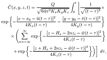
- Starting from the continuity equation one can obtain the advection-diffusion equation through the use of the Reynolds decomposition to separate the mean components for the concentration and the velocity fields. Upon taking averages and substitution of the average fluctuations by Fick’s closure, the desired equation for mean concentrations and an a priori known wind field and with all turbulent characteristics parametrised in a time dependent eddy diffusivity matrix coefficient K is attained. For the current study the eddy diffusion is simplified as locally constant coefficients, which may be justified by the fact that the coefficients vary softly only with changing coordinates and is typical for homogeneous turbulence. For details of the derivation see for instance the textbook by Arya [1].
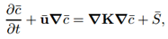 | (1) |
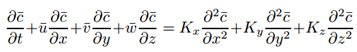 | (2) |
 | (3) |
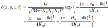 | (4) |
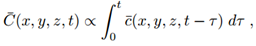 | (5) |
 | (6) |
3. Reflective Boundary Conditions
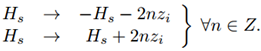
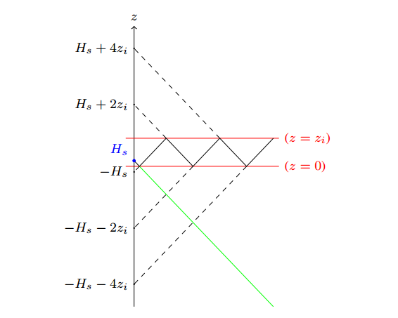
- To justify the mapping of the infinite range z ∈ (−∞, ∞) to the finite z ∈ [0, zi] we first consider a cut of the distribution at z = 0 and z = zi, respectively. Usually the boundary conditions for the pollutant dispersion problem are zero flux or zero concentration at the boundaries, however Fick’s hypothesis suggests there should be a flux across the boundaries. In that sense we copy from observation that the layer until the hight where temperature inversion occurs may be considered at least partially decoupled from the wind flux system beyond. Hence, in an ideally decoupled system the lost contributions should be recovered adopting reflecting boundaries, which intuitively agrees with a simple particle ensemble picture where the pollutant that reaches the ground or the top of the atmospheric boundary layer bounces completely back into the domain. For the distributions that means that even after reflections the Gaussian tails exceeding the allowed domain are mirrored back into the finite range z ∈ [0, zi]. Formally, the reflection on the ground and in the atmospheric boundary layer may be viewed as contributions due to a virtual source in some effective heights to both sides below ground and above the boundary layer [2], those heights are the center of the gaussians formed at the ground and at the top of the atmospheric boundary layer, as exemplified in Figures 1, 2 and 3. The sequences that represent the mirror maxima are
 | (7) |
 | Figure 1. Scheme for the dispersion as if there were no limits in the vertical domain |
 | Figure 2. Scheme for the reflection starting on the ground |
 | Figure 3. Scheme for the reflection starting on the top of the ABL |
 | (8) |
 | (9) |
4. Turbulent Diffusivity Parametrisation
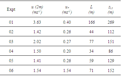
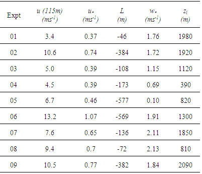
- To validate the proposed model, more specifically to analyse the impact of reflections on the results, turbulent diffusivity was parametrised to represent meteorological conditions of the Hanford [10] and Copenhagen experiment [11].The Hanford experiment is a low source experiment (the height of the source Hs was 2 m) with stable to quasi-neutral conditions. A non-depositing tracer was released with an average rate of Q = 0.3 g/s and release time interval of 30 minutes, except for experiment run 05, where the release time was 22 minutes. The measurements were performed at distances 100 m, 200 m, 800 m, 1600 m and 3200 m from the source. The necessary micro-meteorological data for the parametrisation were provided by the experiment and are presented in Table 1. The height of the stable boundary layer (zi,s) was calculated using the relation zi,s=0.4(u∗L/fc)1/2, where fc=1.46x10⁻⁴ is the Coriolis parameter.
|
|
4.1. Stable Conditions
- The eddy diffusion coefficient for stable conditions proposed by Degrazia and Moraes [7] is based on the diffusion theory of Taylor [20] and the turbulent kinetic energy spectrum [17] and can be computed using the micrometeorological data set from table 1.
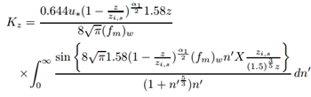 | (10) |
4.2. Convective Conditions
- The eddy diffusion coefficient for convective conditions proposed by Degrazia and Moreira [8] is also based on the diffusion theory of Taylor and the turbulent kinetic energy spectrum and can be computed using the micro-meteorological data set from Table 2. Considering α = x, y, z and i = u, v, w, the eddy diffusion coefficient for convective conditions is
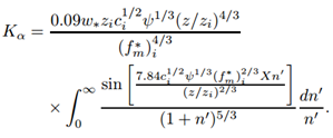 | (11) |
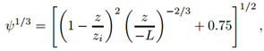 | (12) |
4.3. Wind Speed Profile
- In the further, we introduce a simplification, without imposing restrictions on our numerical findings. We assume, that our coordinate system has its x-axis aligned with the average wind speed, which is to a good approximation horizontal with respect to the Earth’s surface. In order to determine the velocity field u=U(z)x with x a unit vector, we need to fix the vertical wind speed profile. The latter has been parametrised following Monin-Obukhov’s similarity theory manifest in the so-called OML-model [3], where close to the surface and because of its roughness, there is a raising profile, whereas sufficiently far from the surface the wind speed remains approximately constant. If zb = min(|L|, 0.1zi), then
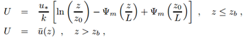 | (13) |
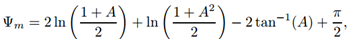 | (14) |
5. Validation of the Model
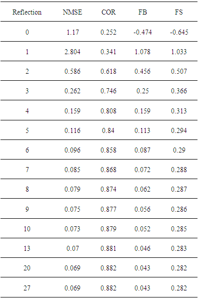
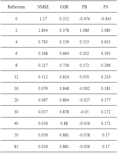
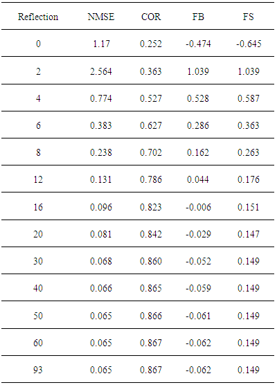
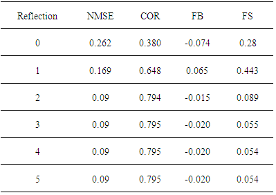
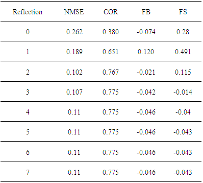
- To simulate the results, it was used the complete data set of the Hanford experimental data, except those for the distances x = 100 m and x = 200 m and the complete data set of the Copenhagen experimental data. The comparison of observed (Co) against predicted (Cp) concentrations for a variety of reflection parameter ωb,g and number of reflections is shown in figures 4, 5, 6 and 7 for the Hanford experiment and in figures 8, 9, 10 and 11 for Copenhagen.The corresponding statistical indices [12], i.e. the normalized mean square error (NMSE), the correlation coefficient (COR), the fractional bias (FB) and the fractional standard deviation (FS) are shown in the tables 3, 4, 5 and 6 for the Hanford experiment 7, 8, 9 and 10 for Copenhagen.A general comment is in order here, although the afore mentioned statistical evaluations are similar to those from parametric inference procedures, their interpretations are different in the present context. In parametric inference the best estimates for parameters were attained for NMSE → 0, but in the present consideration a deterministic model is compared to a relatively small data set from a stochastic phenomenon, so that one does not expect vanishing values for this error. Further, the correlation coefficient does not converge to unity, recalling that the observed data are one sample out of a distribution for a specific situation, that are parametrised using their specific micro-meteorological data. The fractional bias may be interpreted in terms of model fidelity, significant deviations from zero indicate, that the model lacks some relevant physical features.
5.1. Hanford Experiment
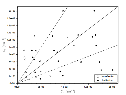 | Figure 4. Scatter plot for observed (Co) and predicted (Cp) concentrations for none and 1 reflection with the parameters ωg = 1.0 and ωb = 1.0 for the Hanford experiment |
|
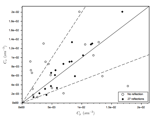 | Figure 5. Scatter plot for observed (Co) and predicted (Cp) concentrations for none and 27 reflections with the parameters ωg = 0.01 and ωb = 0.01 for the Hanford experiment |
|
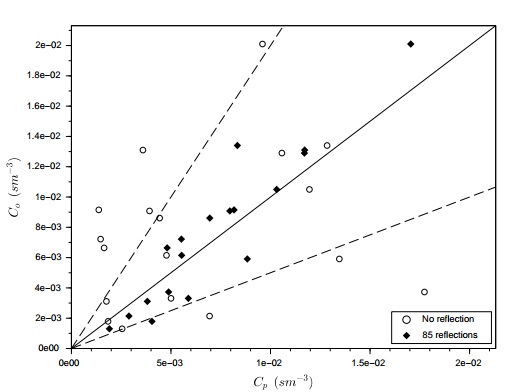 | Figure 6. Scatter plot for observed (Co) and predicted (Cp) concentrations for none and 85 reflections with the parameters ωg = 0.003 and ωb = 0.003 for the Hanford experiment |
|
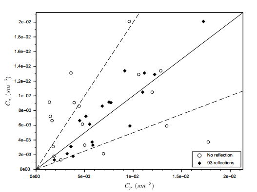 | Figure 7. Scatter plot for observed (Co) and predicted (Cp) concentrations for none and 93 reflections with the parameters ωg = 0.01 and ωb = 0.003 for the Hanford experiment |
|
5.2. Copenhagen Experiment
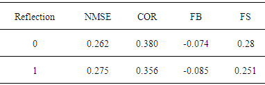
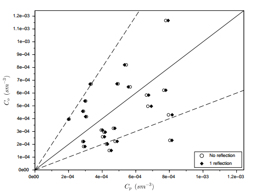 | Figure 8. Scatter plot for observed (Co) and predicted (Cp) concentrations for none and 1 reflection with the parameters ωg = 1.0 and ωb = 1.0 for the Copenhagen experiment |
|
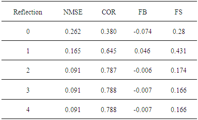
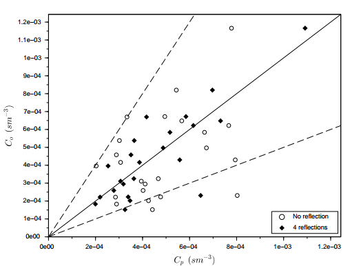 | Figure 9. Scatter plot for observed (Co) and predicted (Cp) concentrations for none and 4 reflections with the parameters ωg = 0.2 and ωb = 0.2 for the Copenhagen experiment |
|
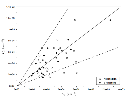 | Figure 10. Scatter plot for observed (Co) and predicted (Cp) concentrations for none and 5 reflections with the parameters ωg = 0.15 and ωb = 0.2 for the Copenhagen experiment |
|
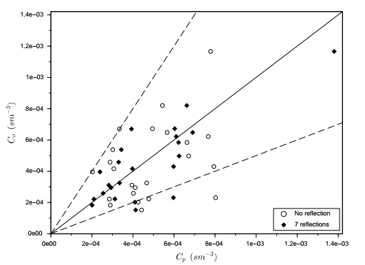 | Figure 11. Scatter plot for observed (Co) and predicted (Cp) concentrations for none and 7 reflections with the parameters ωg = 0.1 and ωb = 0.3 for the Copenhagen experiment. |
|
6. Conclusions
- The present work can be considered an attempt to incorporate stochastic aspects in a deterministic model, i.e. the dispersion of pollutants in the atmospheric boundary layer modelled by the deterministic advection-diffusion equation. The effective boundary layer height may vary according to the turbulent flow dynamics it incorporates hence the boundary layer should have stochastic aspects. A more realistic flow may be thought of as a superposition of various boundary layer problems but with different effective boundary layer heights. So far the intent was to evaluate the contribution of virtual sources superimposing them such as to mimic a finite size sample of a distribution from different boundary layer height realisations.A variety of trials have shown that partial reflection on the boundary layer horizon and the ground obtain the most significant correlations between model and data suggesting that effects on boundary are essential to model dispersion processes in the atmospheric boundary layer, even though the values for the reflection parameters were established ad hoc. This improvement in the solution can be associated with the fact that the deterministic equation predicts only mean values of an unknown distribution and is not capable to predict all stochastic properties, which in our case were modelled by the effects of the considered reflections. Moreover, the model does not consider deposition and adsorption on the ground, but the fact that concentration and vertical concentration fluxes are different from zero on the ground level one may reason, that the parameter ωg is somehow incorporating these properties.
ACKNOWLEDGEMENTS
- This work was supported by Linhares Geração SA, Coordination for the Improvement of the Higher Level Personnel (CAPES - Brazil) and National Council for Scientific and Technological Development (CNPq - Brazil).