-
Paper Information
- Next Paper
- Previous Paper
- Paper Submission
-
Journal Information
- About This Journal
- Editorial Board
- Current Issue
- Archive
- Author Guidelines
- Contact Us
American Journal of Environmental Engineering
p-ISSN: 2166-4633 e-ISSN: 2166-465X
2016; 6(4A): 20-27
doi:10.5923/s.ajee.201601.04

Analytical Solution for a Pollutant Dispersion Model with Photochemical Reaction in the Atmospheric Boundary Layer
 Abstract
 Reference
 Full-Text PDF
 Full-text HTML
Guilherme Jahnecke Weymar1, Bardo Ernst Josef Bodmann1, Daniela Buske2, Jonas da Costa Carvalho2, Marco T. M. B. Vilhena1
1Pos-Graduate Program in Mechanical Engineering, Federal University of Rio Grande do Sul, Porto Alegre, Brazil
2Pos-Graduate Program in Mathematical Modelling, Federal University of Pelotas, Pelotas, Brazil
Correspondence to: Guilherme Jahnecke Weymar, Pos-Graduate Program in Mechanical Engineering, Federal University of Rio Grande do Sul, Porto Alegre, Brazil.
| Email: |  |
Copyright © 2016 Scientific & Academic Publishing. All Rights Reserved.
This work is licensed under the Creative Commons Attribution International License (CC BY).
http://creativecommons.org/licenses/by/4.0/

This paper presents an analytical solution for the three-dimensional advection-diffusion equation applied to the dispersion of pollutants that form in the Atmospheric Boundary Layer (ABL). Some substances, when emitted in ABL suffer photochemical reactions producing secondary pollutants, so that a source term is included in the advection-diffusion equation to represent this reaction. The model was applied to simulate the dispersion and transport of ozone (O3) produced by photochemical reactions from nitrogen dioxide (NO2), pollutant emitted by burning fossil fuels by automotive vehicles. The pollutant concentration fields obtained by the proposed solution are compared with mixing ratio data obtained by monitoring the air quality in the metropolitan area of Porto Alegre. From the analysis of the results one verifies that the inclusion of the term proposed to represent a photochemical reaction of a reactive pollutant allows to predict ozone concentrations in the ABL.
Keywords: Advection-diffusion equation, Photochemical reaction, Analytical solution, GILTT method
Cite this paper: Guilherme Jahnecke Weymar, Bardo Ernst Josef Bodmann, Daniela Buske, Jonas da Costa Carvalho, Marco T. M. B. Vilhena, Analytical Solution for a Pollutant Dispersion Model with Photochemical Reaction in the Atmospheric Boundary Layer, American Journal of Environmental Engineering, Vol. 6 No. 4A, 2016, pp. 20-27. doi: 10.5923/s.ajee.201601.04.
Article Outline
1. Introduction
- The interest in preserving the air quality is growing considerably in recent years due to increased emission of pollutants in the atmosphere caused by the increase of industrial development and the burning of fossil fuels by automotive vehicles. Thus, to control the air quality one needs an interpretive tool, such as a mathematical model that is able to link the cause (pollution source) with the effect (pollutant concentration distribution). The use of certain mathematical models in addition to the observed measurements produce a qualitative as well as quantitative progress in the management of air pollution, because the models allow a more complete description of the development of the transport phenomenon with respect to spatial distributions and forecast the concentration distribution evolution [1], whereas measurements are typically restricted to a small set of points.Today, one can say that one of the biggest problems caused by air pollution in urban areas are caused by photochemical oxidants, these are formed in the atmosphere by reaction between volatile organic compounds (VOC's) and nitrogen oxides
 in the presence of sunlight, where the principal component is ozone (O3). Therefore, the pollutant of interest in this work is ozone, which is classified a secondary pollutant that appears as a bluish reactive gas and approximately 1.6 times heavier than oxygen molecules. The oxidizing character of this gas can cause extensive damage to fauna and flora. Furthermore, ozone contributes to the greenhouse effect since the compound presents an absorption band at
  [2].According to [3], cars are the main sources of emissions of ozone precursors. Even knowing the complexity of atmospheric chemistry, when the atmosphere has predominance of nitrogen compounds the formation of tropospheric ozone is well known. However, when there is the presence of hydroxyl radicals
  and hydrocarbons these cause an atmospheric disequilibrium, resulting in increased ozone formation.Thus, this work presents an analytical solution for three-dimensional advection-diffusion equation applied to the dispersion of pollutants formed from a photochemical reaction in the Atmospheric Boundary Layer (ABL), the resolution of the problem is done with the use of techniques of Laplace transform and GILTT (Generalized Integral Laplace Transform Technique) [5].
2. Photochemical Reaction and Ozone Production
- Ozone
 performs a fundamental role in stratospheric chemistry, because it reacts with ultraviolet light behaving as a protective shield against the harmful effects of radiation. However, ozone is a highly reactive and toxic species, and when present in the troposphere has prejudicial effects to many living beings.According to [4], the most important reaction in the production of ozone in the atmosphere is between atomic oxygen and molecular:
 | (1) |
 which removes the energy of reaction and stabilizes
  At high altitudes (above 20km), oxygen atoms are produced by photo dissociation of molecular oxygen by absorption of deep ultraviolet radiation. At lower altitudes, where there is only radiation with wavelengths longer than 290nm, the only source of atomic oxygen is the photo dissociation of nitrogen dioxide:
 | (2) |
 has a wavelength between 290nm and 430nm. An ozone removal process is its reaction with nitric oxide:
 | (3) |
 consuming a molecule of
  A reaction that converts the
  to
to  without consuming the molecule
  may cause accumulating of ozone. This reaction occurs in the presence of hydrocarbons. In particular, peroxy radicals
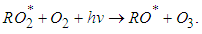
  where "R" is an alkyl group and produced in the oxidation of hydrocarbon molecules react with the
  to form the
  allowing an increased production of ozone:
 | (4) |
 | (5) |
 | (6) |
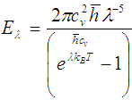
 is the speed of light,
  is Planck's constant,
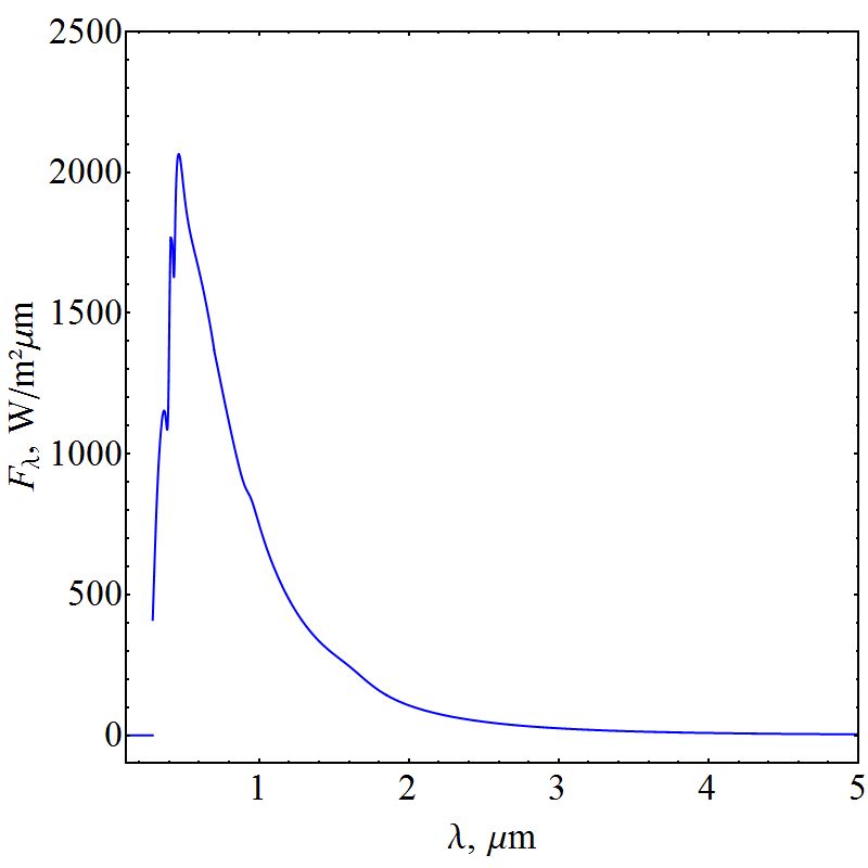
 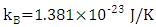 is Boltzmann constant. From equation (6), a curve fitting was performed using the method of least squares and a Padè approximation 4-5 and 4-6. Figure 1 shows the graph of the set of the adjusted solar irradiance function:
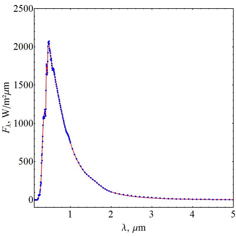 | Figure 1. Function of Solar Spectral Irradiance |
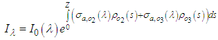
 | (7) |
 is the spectral radiance along a path in the direction
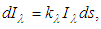
  is called the extinction coefficient. The extinction coefficient is represented by
 | (8) |
 is the density of gases (which may vary along the path
  and
and  is the extinction cross section at the wavelength
  Extinction is the sum of the cross sections of absorption and scattering
 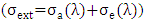 . In this study, we considered only the absorption of gases, thus
  and therefore:
 | (9) |
 and
and  are the cross-section of absorption and the density at the height
  of gas i, respectively (N is the number of gases that composes the atmosphere).According to [8], the spectrum region from
  to
to  most of the solar radiation is absorbed by gases
  and
and  Therefore, to calculate the solar radiation reaching the PBL, one considers only the oxygen and ozone absorption:
 | (10) |
 | Figure 2. Cross section of oxygen absorption |
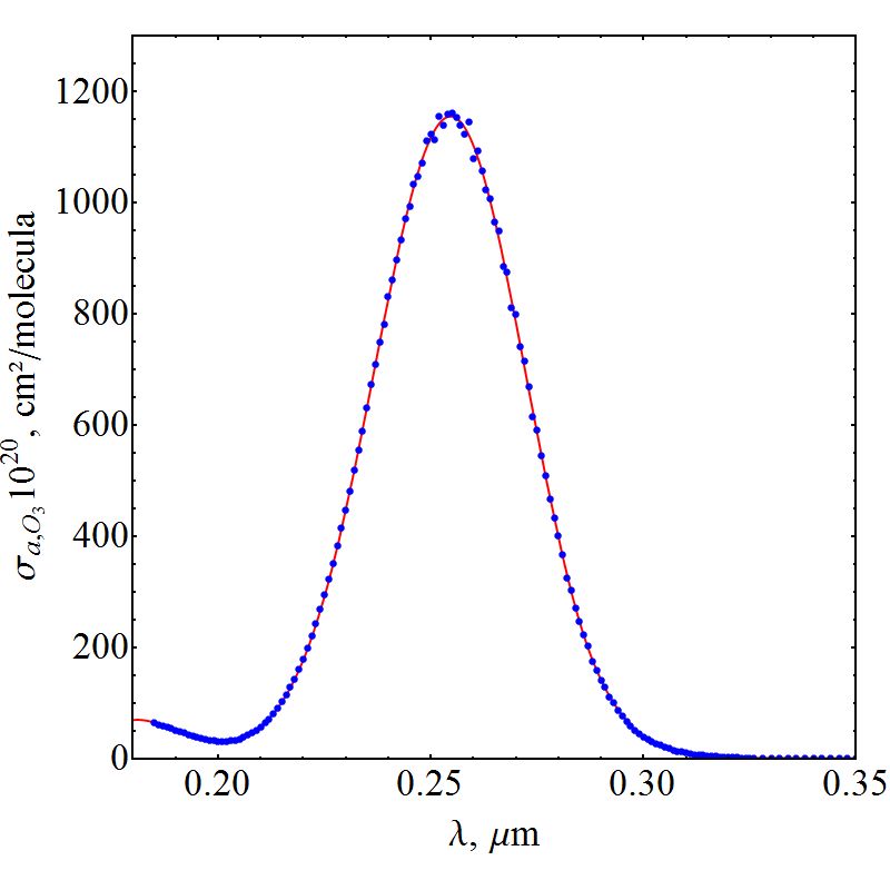 | Figure 3. Cross section of ozone absorption |
 | (11) |
 | Figure 4. Solar Spectral Irradiance Function that reaches ABL |
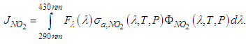
 According to [11], the rate (or frequency) of atmospheric photolysis (J) are of fundamental interest in the study of atmospheric chemistry processes.Photo dissociation of the
  is described as a first order process [9], represented by:
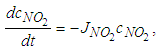 | (12) |
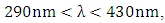 the frequency of photolysis of
  is represented by the coefficient
  was calculated as follows [27],
 | (13) |
 is the local flux, that is, the amount of light available in the atmosphere,
  is the cross section of absorption of the molecule, or it is the intensity of light available at a given wavelength that the molecule can absorb and
  (molecule/photon) is the quantum yield, that represents the probability with which a compound absorbs light of a certain wavelength.For simplicity one considers the absorption cross section and the quantum yield
  depending only on the wavelength
  and with the available data from [12], one obtains
  and
and  as shown in Figures 5 and 6, respectively.
 | Figure 5. Absorption cross section function of NO2 |
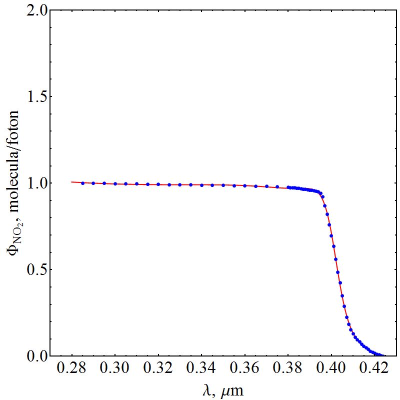 | Figure 6. Quantum yield function of NO2 |
 | (14) |
3. Solution of Three-Dimensional Advection-Diffusion Equation
- To model the ozone concentration distribution the transient three-dimensional advection-diffusion equation was employed and a photochemical reaction term added (first-order process), this term is the photo dissociation
 in
in 
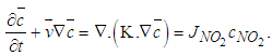 | (15) |
 the average concentration of the pollutant (ozone),
  the average wind speed,
  the matrix of diffusion coefficients
 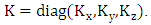 The domain of interest is a cube with dimensions
  and h, where h is the height of PBL. Equation (15) is subject to zero-flow boundary conditions on the faces of the cube, zero initial concentration (at t = 0) and source condition
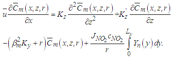
  Observe that the production of ozone takes place only by photochemical reactions. To solve the proposed problem, we apply the spectral method in the variable y, that is, the pollutant concentration is expanded in a series with terms of eigenfunctions of an associated Sturm-Liouville problem and making use of the integral operator
  thus transforming the equation (15) in a transient system of two-dimensional advection-diffusion equations, and the following simplifying assumptions: The advection is dominant along the x-axis direction
  the wind direction is oriented in the
  and for the coefficient of lateral turbulent diffusivity,
  one obtains the following equation:
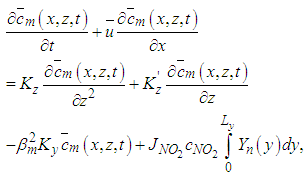 | (16) |
 | (17) |
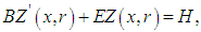 | (18) |
 is the vector of components
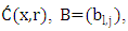
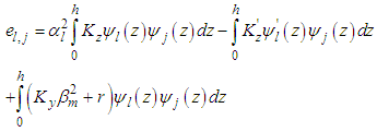
 are arrays whose entries are:
 | (19) |
 | (20) |
 | (21) |
 so that
  is well established. To obtain
  one applies the inverse Laplace transform in
  where the inversion is done numerically by the use of Gauss quadrature.Once
  is known, the final solution of the advection-diffusion equation (15) is given by the equation:
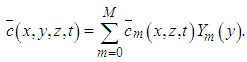 | (22) |
4. Validation against Experimental Data
- For an adequate prediction of transport and diffusion models in the atmosphere validation against experimental data are of need. To this end besides some measured data also topographical properties and typical meteorological conditions of the area to be analyzed [25] shall be employed.To this end, this section presents the parameterization of turbulent diffusion coefficients, wind profile, the observed data used in this study and the numerical results obtained with the model.
4.1. Physical Model Parameterization
- In atmospheric diffusion problems, the choice of a turbulent parameterization represents a fundamental decision to model the dispersion of pollutants. The parameterization of turbulence is an approximation of nature in the sense to try to represent the physical phenomena by parametrized expressions. The reliability of a model is strongly related to the way in which the parameters are calculated and related to the PBL [26].
4.1.1. Turbulent Diffusion Coefficients
- We used the following vertical and lateral diffusion coefficients as suggested by [14] and derived from [15] for unstable conditions

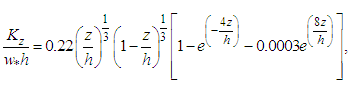 | (23) |
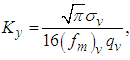 | (24) |
 is the Eulerian standard deviation of longitudinal turbulent velocity given by:
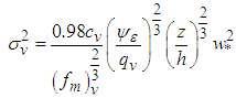 | (25) |
 is the vertical component of the normalized frequency of the spectral peak,
  is the stability function,
  is molecular dissipation rate function expressed by [16], [17]:
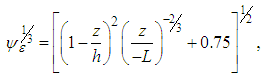 | (26) |
4.1.2. Wind Profile
- In a first approximation and to describe the wind field for the simulations of the dispersion of pollutants, the equation used for wind parameterization is described by a power law expressed by [18],
 where
where  are the horizontal average wind speeds in the heights
  respectively, and
  is an exponent which is related to the intensity of turbulence [19].
4.2. Observed Data
- The FEPAM (“Fundação Estadual de Proteção Ambiental Henrique Luiz Roessler”) is a Brazilian institution responsible to evaluate, monitor and disseminate information about environmental quality. This organization has a monitoring station in the Metropolitan Region of Porto Alegre (MRPA). In January of 2006, a monitoring campaign of air quality in the MRPA was performed, and the measurements among others yielded the mean concentrations of ozone and nitrogen dioxide. The location of the monitoring station close to the town of Esteio is represented by the red dot in Figure 7.
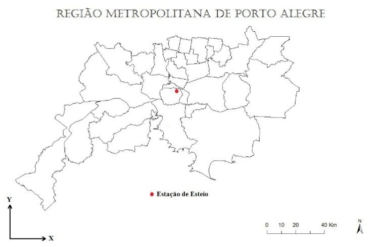 | Figure 7. Location of the monitoring station in Esteio (FEPAM) |
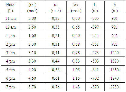
 is the reference speed (m / s),
  is the friction velocity (m / s),
  is the length of Monin-Obukhov (m),
  is the convective vertical speed scale (m / s) and h is the PBL height (m).
|
 | (27) |
 is the constant of Von-Kármán
  and
and  [21]. The speed friction
  is obtained by
 where
where  (reference height) and
  is the wind speed. The CLP height h is obtained from the relationship
  [22], [23], wherein
  (Coriolis force).
4.3. Numerical Results
- To perform statistical comparisons between the model and observed data we consider the set of statistical indices described by [24] and defined as follows:
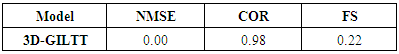
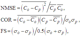 where the subscripts o and p refer to the observed and predicted concentration, respectively, and the bar represents the mean value. The best results are expected to have values close to zero for NMSE and FS indexes, and close to 1 for the correlation index COR.Table 2 presents the results of statistical indexes, where one observes that predicted concentrations of the model reproduces satisfactorily the experimentally findings.
|
 simulated
  and observed
  data. One observes fairy good agreement between the predicted and observed concentrations in the period from 11 am to 7 pm to January 05, 2009.
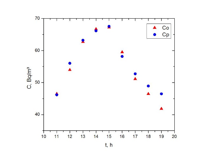 | Figure 8. Comparison between the mean hourly concentrations during the days of January simulated and observed for Esteio station (FEPAM) |
5. Conclusions
- This paper presents a new analytical representation for the solution of the advection-diffusion equation with small error in the numerical inversion of the inverse Laplace transform, for the dispersion problem of a secondary pollutant. The model in question considers photochemical reaction of a primary pollutant released into the atmosphere which gives rise to ozone prediction. Analytical solutions are of fundamental importance to understand and describe physical phenomena, as they take into account explicitly all the parameters involved in the problem, so that their influence can be reliably investigated. In the proposed model, a photochemical reaction of a primary pollutant in the atmosphere is considered in order to improve forecasting and understanding the dispersion of ozone formed in the planetary boundary layer. Even with adopted simplifications presented in this work, the model was able to reproduce the behavior of the ozone concentration during the period from 11 am to 7 pm with a fairly good fidelity.
ACKNOWLEDGEMENTS
- The authors thank CAPES (“Coordenação de Aperfeiçoamento de Pessoal de Nível Superior”) and CNPq (“Conselho Nacional de Desenvolvimento Científico e Tecnológico”) for financial support.