1. Introduction

The present work shows a model based on an advection-diffusion equation (A-D), which describes the dispersion of pollutants in the atmosphere. The principal objective of the forthcoming discussion is to consider time dependence in the wind field and in the eddy diffusivity to get more realistic results of the dispersion phenomenon with moving sources. To attain this objectives, we use an idea inspired by Adomian’s decomposition method [1-3]. Thus, the original advection-diffusion equation which describes the problem is cast in a set of recursive equations, where each one is solved by the GILTT (Generalized Integral Transform Technique) method. A complete review of the GILTT method is given in [15] and references therein.

The results obtained with the model are compared with measurements from the OLAD campaign (Over-Land Alongwind Dispersion). This experiment was conducted in the period of 8 – 25 September, 1997 at the U.S. Army Dugway Proving Ground (DPG) West Desert Test Center (WDTC). The OLAD experiment made use of continuous release of a known quantity of tracer gas (sulfur-hexafluoride, SF6) along a line perpendicular to the prevailing wind direction. These releases were accomplished using either an aircraft or truck mounted dissemination system. The aircraft-mounted disseminator line source of 20-km length and at an altitude of 100 m above ground level (AGL), while the truck-mounted disseminator line source was of 10 km length and at 3 m AGL. The line-source tracer cloud generated during each release advected downwind towards three lines of surface-mounted samplers and one aircraft-mounted sampler. Each surface sampling line, located 2 to 20 km downrange of the dissemination line, consisted of 15 whole-air samplers spaced at 100-m intervals. The whole-air samplers reproduced time-averaged (15 min) tracer gas concentrations [4].

The results presented in this work refer to a simulation of day 12 of September, denoted OLAD 5. In this experiments the release is performed by truck-mounted disseminator. The data of concentration considered for simulation comparison were of the sampler located in the route Foxtrot 2 km away from the release location. To this end the line source was represented by a finite number of point sources.

2. The Analytical Solution

The advection-diffusion equation is a deterministic approach to dispersion of pollutants in the atmosphere. It is obtained by mass conservation combined with first order close (K-Theory) [5]:

(1)

Here denotes the mean concentration of a passive contaminant; are the cartesian components of the mean wind speed in the direction x, y and z, respectively; and are the eddy diffusivities. For convenience we align the predominant wind direction with the direction of the x coordinate, and equation (1) simplifies to

(2)

The space-time domain is given by and and equation (2) is subject to the following boundary and initial conditions:

Recalling that the line source was discretised, so that each individual point source was represented by a generic source condition,

with being the emission rate, the height of the atmospheric boundary layer, the height of the source, and are domain limits in the x and y-direction far from the source and represents the Dirac delta function.

In order to construct a solution, first we separate time-dependent wind field and time-dependent eddy diffusivity contributions from their time averaged values:

(3a)

(3b)

(3c)

(3d)

where and are the time averages. Upon inserting this assumptions in equation (2) yields:

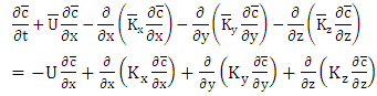(4)

According to the idea of the decomposition method the solution of (4) is written as a truncated expansion:

(5)

These new degrees of freedom for each component may now be used to decompose (4) into a set of advection-diffusion equations, that together form a recursive scheme:

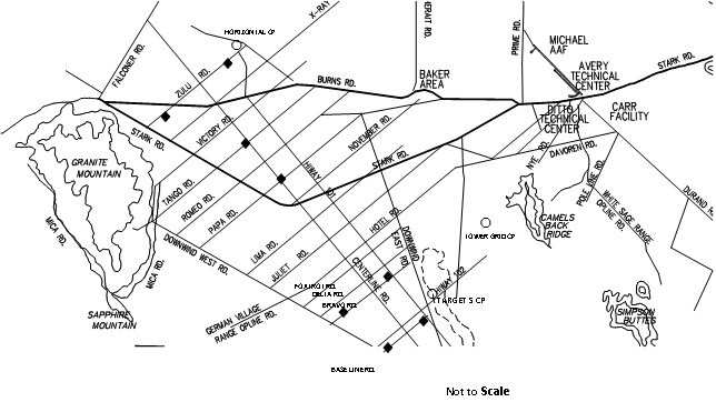Figure 1. OLAD test site at Dugway Proving Ground showing the locations of dissemination lines, sampling lines, and meteorological measurement sites [4]

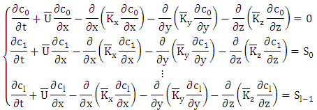Here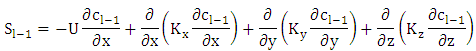

Note, that the decomposition procedure is not unique. Our choice for reshuffling term with the specific form of source terms is justified because it allows to solve the resulting recursive system analytically by the GILTT method. Further, the time dependence of the eddy diffusivity and wind field in the proposed solution is entirely accounted for in the source term, which is constructed from the solutions of previous recursion steps and thus are known. Moreover, the recursion initialisation satisfies the boundary conditions of the original problem, whereas all the subsequent recursion steps satisfy homogeneous boundary conditions. Once the set of problems is solved, the solution of equation (5) is well determined. A remark on the truncation is in order here, the accuracy of the results may be controlled by the proper choice of the number of terms in the solution series.

2.1. The GILTT Method

The equations of the set of recursive equations are solved, by applying initially the Laplace transform in the t variable, which leads to

(6)

where denotes the Laplace transformed concentration in the t variable

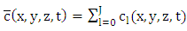
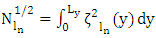
Upon making use of the expansion of the concentration series with respect to the y coordinate:

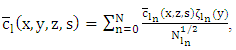(7)

where and are the eigenfunctions of the associated Sturm-Liouville problem with eigenvalues one may proceed further with the unknown coefficient for the dimensionally reduced problem. To this end (7) is replaced in (6) and after projecting out orthogonal components yields

(8)

where

The afore mentioned procedure may be repeated for the z coordinate with the eigenfunctions of the associated Sturm-Liouville problem, and are the respective eigenvalues. Again, projecting out orthogonal components reduces the original equation by one further dimension and the equation is cast in matrix form for the dimension where the coordinate axis is aligned with the wind direction:

(9)

Here is the vector of the coefficients and

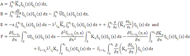
Equation (9) it is solved by order reduction with and 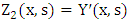, so that the remaining problem to be solved is

(10)

with

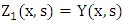
To solve problem (10) one may employ the steps detailed in reference [16], where a combined Laplace transform technique and diagonalization procedure was proposed. The recursive problem reads then

(11)

where for the recursion initialisation and thus

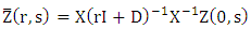whereas for the other equations so that

where denotes the Laplace Transform of vector Here X is the matrix of the eigenvectors of matrix M and is its inverse. The matrix D is the diagonal matrix of eigenvalues of the diagonalised problem, where the entries of the matrix (rI + D) have the form {s + dn}. After Laplace transform inversion of (12), we get:

where is the diagonal matrix with components Further, the unknown constant vector is given by (initialisation) or (recursion), respectively.

Once these coefficients are evaluated one can construct the analytical solution of problem (7) applying the inverse Laplace transform definition. This procedure yields a result in analytical representation:

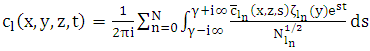(12)

For numerical purposes and to overcome the difficulty of evaluating the line integral appearing in Eq. (12), one may approximate the integral by a Gaussian quadrature scheme:

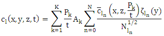Here and are the weights and roots of the Gaussian quadrature scheme tabulated as for instance tabulated in the book of Stroud and Secrest [21].

3. Results

The solution of the considered model may be evaluated against the OLAD experiment [4]. To this end the dataset of the 12^th September 1997, where sulfur-hexafluoride (SF6) was released by a truck mounted disseminator at 3 m above ground level and following the Bravo route for 10 km. The beginning of the emission was at 6 hours and 58 minutes with duration of 10 minutes. According to reference [7] this experiment has the characteristic of low wind speed less or equal 3.5 m/s. Further, the planetary boundary layer showed a stable condition during the sampling period, as classified by the Monin-Obukhov lengths presents in the Table (1).

The whole-air samplers produced time-averaged (15-min) tracer gas concentrations, that are referenced by the respective fifteen analysers (LC101-LC115) located along the route Foxtrot with a distance of 2 km “parallel” to the Bravo Route. We used ten point source to reliable represent the experiment’s line source, and in each source the release duration was Thus the concentration in each sampler is defined by

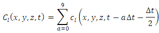where a denotes the displacement centred line segment source, as shown in Figure 2.

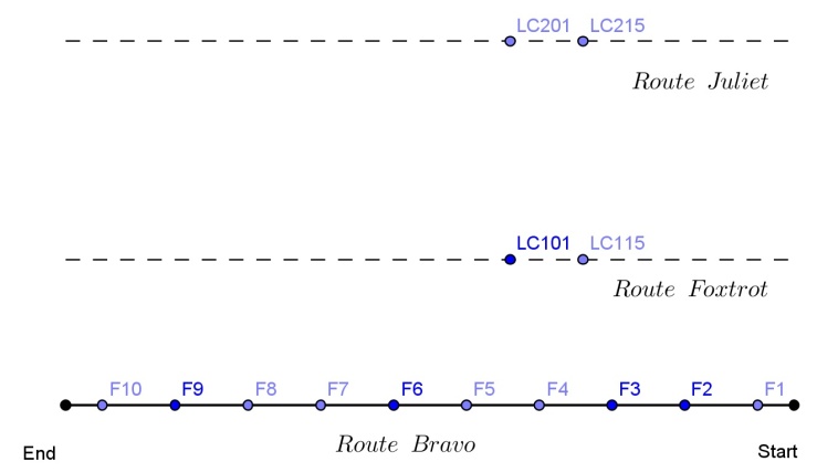Figure 2. Representation of the ten point source

3.1. Simulation Source

While the real experiment used a continuous line source to dissemination the tracer, for convenience we used in the simulations a finite number of point source to represent the problem. Figure 2 shows the implemented representation of this approximation.

3.2. Parameterisation

In atmospheric diffusion problems, the choice of the turbulence parameterisation is a fundamental decision to adequately model the dispersion process. From the physical point of view the turbulence parameterisation is a phenomenological approach for a complex dynamics that up to date is far from being described in terms of a consistent non-linear theory, so that dimensional arguments and similarity conceptions provide a mathematical model that is being used as a surrogate for the terms that should come from the afore mentioned unknown theory. Hence, the reliability of each model strongly depends on the way turbulent parameters are calculated and related in the context of current understanding of the ABL [11]. In stable conditions of the boundary layer the vertical eddy diffusivity can be formulated as [9]

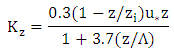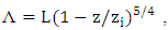where whereas Degrazia et al. proposed for a stable boundary layer an algebraic formulation for the eddy diffusivity in the x and y direction according to [8],

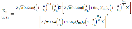where is the frequency of the spectral peak, 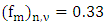is the frequency of the spectral peak in the neutral stratification [20], [17]) is the local Monin-Obukhov length, 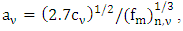where is the friction velocity and represents the non-dimensional distance. The wind speed profile can be describe by the power law [12]

where are the horizontal wind velocity at height and The power parameter is related to the intensity of turbulence.

3.3. Numerical Results

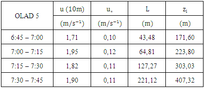
In the experiment five of OLAD the beginning of the emission was at 6 hours and 58 minutes. We used the meteorological data of the first hours to simulate the dispersion with the proposed model. The data presentd in Table 1 were calculated in [8] based on the dataset of reference [4]. The data and represent the wind speed in 10 meters, the friction velocity, Monin-Obukhov length and the height of the planetary boundary layer, respectively.

Table 1. Meteorological conditions of OLAD 5 [8]

The concentrations obtained with the simulation in this work are for the period of 6:45 – 7:45 and we used the concentrations observed in the first sampling line of the experiment for comparison. In all fifteen analysers the convergence of the series (5) occurred after six terms. In Table 2 we present the numerical convergence of the results for sampler LC115.

Table 2. Concentration of the LC115 with five recursion steps

The first sampling line located in the route Foxtrot have fifteen samplers denoted LC101 to LC115. In Table 3 concentration results observed in the experiment (CO) and concentrations predicted by model proposed (CP) are shown.

Table 3. Tracer concentration for the fifteen samplers of experiment five of OLAD and model prediction

Although the analysers LC101, LC102 and LC103 present results in disagreement between experiment and model, the results obtained with the model describe with efficiency the dispersion phenomenon. Low quality observed concentrations presents in the afore analysers are justified either by inaccuracy of samplers or by an experimental failure.

In Figure (3) one can check the concentration for the fifteen analyser of the Foxtrot route.

Figure 3. Observed and predicted concentration

3.4. Statistical Results

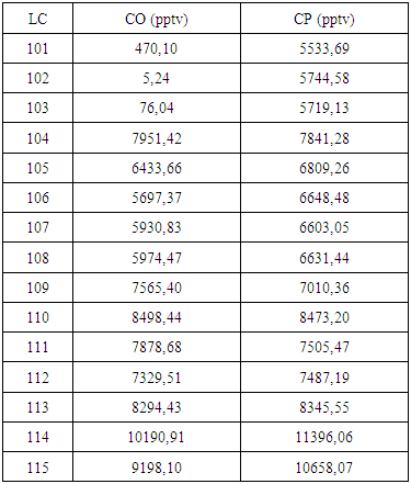
The comparison between the observed (C_o) and predict (C_p) data concentration shown in Table (3) were analysed statistically [13]

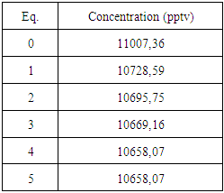
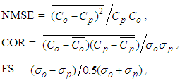where NMSE, COR and FS represent the normalized mean square error, correlation coefficient and fractional standard deviations, respectively. Due to a stochastic phenomenon, that is being simulated by a deterministic model a small NMSE and a correlation coefficient beyond ~0.8 (but less than 1) indicating an acceptable solution (see Table 4).

Table 4. Statistical comparison between observed and predict concentration

Figure (4) confirms the agreement of the model results with the data of the experiment of OLAD.

Figure 4. Observed (CO) and predict (CP) scatter plot

4. Conclusions

The present work is a continuation in a sequence of implementation that as a general problem treat the pollutant dispersion in the atmosphere considering physically relevant meteorological scenarios and a diversity of pollution sources. Progress in relation to previous works considers the implementation of time dependence in the eddy diffusivity and the field wind, respectively. Most of the analytical problems found in the literature make use of fixed sources, however, a considerable amount of pollutant release is due to sources in motion. The model was validated using data from an experiment with moving source, the OLAD campaign. In this experiment a tracer substance was emitted from a facility mounted on a truck that run on the route Bravo along 10 km and thus represents a time dependent line source. For convenience this line source was approximated by a sequence of point sources, between two subsequent sources the emission was delayed by a time interval, in agreement with the experimental setup. Trials with different discretisations have shown us that the present implementation allows to simulate fairly well the dispersion of the experiment.

To this end the advection-diffusion equation was solved by a combination of a decomposition method, and the Generalised Integral Laplace Transform Technique (GILTT). While the first part of the solution method produces a recursive set of equations, where each of the equations have a known solution by GILTT. We also analysed stability of the procedure which showed that only a small recursion depth is necessary in order attain an acceptable accuracy (Table 2) for the simulated concentration as measured in analyser LC115. Results for the other samplers are comparable in quality with the previous one.

The results of concentration obtained with the model and the concentrations observed in the experiment show similar behaviour and one can conclude that the proposed model describes satisfactorily the phenomenon. Disagreement in some of the values in three of the samplers may be attributed either to atypical behaviour of meteorological conditions limited to the time interval of emission and measurement. Moreover there may be a discrepancy because of the fact that the phenomenon is stochastic whereas the model is deterministic and thus reproduces only average values, while the measured data are one sample of an unknown distribution. Also malfunction of the instruments may not be excluded and those topics will be analysed in future works.

ACKNOWLEDGEMENTS

The authors thank CAPES (Coordenação de Aperfeiçoamento de Pessoal de Nível Superior) and FAPERGS (Fundação de Amparo à Pesquisa do Estado do Rio Grande do Sul) for the partial financial support this work.