Igor C. Furtado, Bardo E. J. Bodmann, Marco T. Vilhena
Pos-Graduate Program in Mechanical Engineering, Federal University of Rio Grande do Sul, Porto Alegre, RS, Brazil
Correspondence to: Igor C. Furtado, Pos-Graduate Program in Mechanical Engineering, Federal University of Rio Grande do Sul, Porto Alegre, RS, Brazil.
| Email: |  |
Copyright © 2016 Scientific & Academic Publishing. All Rights Reserved.
This work is licensed under the Creative Commons Attribution International License (CC BY).
http://creativecommons.org/licenses/by/4.0/

Abstract
The dispersion of pollutants in the atmospheric boundary layer is a stochastic process but many approaches make use of deterministic models, such as the advection-diffusion equation, that determines average values. Comparison between observation and model prediction show a significant spread of values due to the stochastic character of the pollution dispersion phenomenon. Measured data though represent only one sample of an unknown distribution. Thus, the present article is a first attempt to reconstruct at least some of the pollutant concentration distribution properties from the comparison of deterministic predictions to observed concentrations under specific micro-meteorological conditions. The experimental data are the findings of the Copenhagen campaign. We show the scatter plot of observed versus predicted ground level concentrations from which distributional properties are extracted by determining the distance of each plot point from the bisector, proposing a parametrization for the probability function and fit the discrete set of data points. The probability density function obtainde from the probability distribution shows a narrow peak centered at zero besides a second smaller but displaced contribution. A reconstructed distribution symmetrically around zero signifies, that the model describes the average values of the distribution with fairly good fidelity and the width could be used as an approximation for the second statistical moment. The distribution which is not centered at the origin indicates either missing physics in the model, or failures in the measuring procedure. The reconstructed distribution with correlation less than one shows the aforementioned stochastic character of the phenomenon. Although applied to a specific experiment and using one deterministic model the reconstruction method is general and can be applied to other scenarios in an analogue fashion.
Keywords:
Dispersion of pollutants, Stochastic phenomenon, Deterministic predictions, Probability density function
Cite this paper: Igor C. Furtado, Bardo E. J. Bodmann, Marco T. Vilhena, On the Reconstruction of Concentration Distributions from Comparison of Deterministic Predictions to Observational Data, American Journal of Environmental Engineering, Vol. 6 No. 4A, 2016, pp. 6-11. doi: 10.5923/s.ajee.201601.02.
1. Introduction
The dispersion of pollutants in the atmospheric boundary layer is a stochastic process which varies unpredictably over a time interval. Although it is a random phenomenon, in many approaches is modeled by deterministic models, in our case given by the advection-diffusion equation, that determine average values.A variety of studies have shown that in almost all cases a significant spread of values in the observed-predicted concentration plot occurs which on the one side may have influences by model uncertainties but on the other hand stems from the stochastic character of the dispersion phenomenon.Independent of the model nature and its predictability, it is noteworthy, that measured data in general may not be repeated with equal micro-meteorological conditions, so that often a measured concentration is only one sample of an unknown distribution, with its related statistical moments.The model choice in favor of the advection-diffusion equation is based on formal progress in solving this equation in an (semi-)analytical fashion and although predicting only average values shows fairly good agreement with measurements. The short coming of lacking information of higher statistical moments in the model is to its simplified closure by K-theory. This theory was extended by parameterizations that besides the vertical eddy diffusion profile also takes into account the changes in the diffusion parametric functions with distance from the pollution source.In this line the present article is a first attempt to reconstruct at least some of the pollutant concentration distribution properties from the comparison of deterministic predictions to observed concentrations for observations with determined micro-meteorological conditions. The same conditions are used for the deterministic dispersion simulations. In principle, the presented procedure may be applied to any other dispersion model, so that in the present discussion, focus is put on the reconstruction procedure and less on the pertinent question as to what is the most appropriate model for describing the phenomenon in consideration.
2. The Model
The model used in this approach is the advection-diffusion equation obtained by combining the continuity equation with Fick’s Law: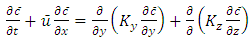 | (1) |
where  is the direction of the mean wind,
  is the mean concentration,
  is the mean wind,
  and
and  are the turbulent diffusion coefficients and in this case
  dependent on the height
  and time
  Equation (1) is subject to the initial condition of zero concentration and zero flow in the contours of the area of interest. The source is
  in
in  where
where  is the rate of emission of the pollutant,
  is the height of the source,
  is the Dirac delta function,
  is characterized by the crosswind coordinate of the source and
  is the height of the boundary layer.The success of a deterministic model is strongly influenced by the way the turbulent parameters are related to the understanding of the phenomenon. The diffusion coefficient, with temporal dependence, derived by Degrazia et al. [1] is based on diffusion theory, statistical Taylor approach and a spectral model of kinetic energy. This methodology derived from convective and moderately unstable conditions, provide diffusion coefficients characteristic described in terms of speed and duration of energy containing eddies and scales can be expressed by algebraic formulation as:
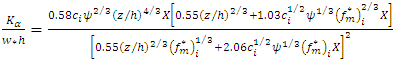 | (2) |
Here 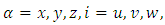 and
and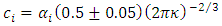
 respectively for
  and
and  [2],
[2],  is the von Karman constant,
  is the normalized frequency of the spectral peak,
  is the height of the atmospheric boundary layer,
  is the convective velocity scale,
  is the non-dimensional molecular dissipation rate function and
  is the non-dimensional travel time, where
  is the horizontal mean wind speed.For horizontal homogeneity the convective boundary layer evolution is driven mainly by the vertical transport of heat. As a consequence of this buoyancy driven ABL, the vertical dispersion process of scalars is dominant when compared to the horizontal. Therefore, the present analysis will focus on the travel time dependent vertical eddy diffusivity. This vertical eddy diffusivity can be derived from Eq. (2) by assuming that
  and
and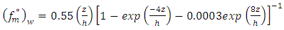 for the vertical component [3].Furthermore, considering the horizontal plane, we can idealize the turbulent structure as a homogeneous one with the length scale of energy-containing eddies being proportional to the convective boundary layer height h. Thus, for the lateral eddy diffusivity we used the asymptotic behaviour of Eq. (2) for large diffusion travel times with
  and
and 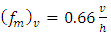 [4].Finally, the dissipation function
  according to [5, 6] has the form
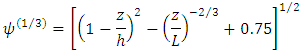 where
where  is the Monin-Obukhov length in the surface layer.
2.1. Results 3D-GILTT
Equation (1) was solved analytically in [7] by combining the idea of the decomposition method and GILTT. Upon applying the idea of the decomposition reduces the advection-diffusion equation with time dependence of the diffusion coefficient into a set of recursive equations depending only on the diffusion coefficient in the spatial variable 
 which is then directly solved by the aforementioned method.Evaluation of the performance of the 3D-GILTT and simulation of the dispersion of contaminants in the atmospheric boundary layer is compared to the performance of the solutions against experimental concentrations of the Copenhagen campaign [8].The vertical wind speed profile used in the simulations is described by the power law that follows
 | (3) |
where  are the average speeds of the horizontal wind at heights
  respectively and
  is an exponent which is related to the intensity of turbulence [9], where according to the author
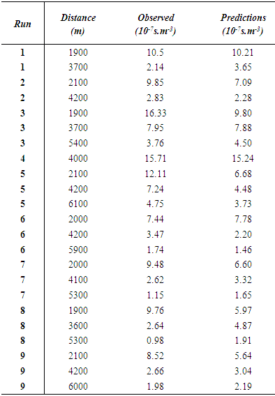
  is valid for a power wind profile in unstable conditions. Table 1 shows the comparison of 3D-GILTT simulated results against experimental data.
Table 1. Pollutant concentrations for nine runs at various positions of the Copenhagen experiment and model prediction by the 3D-GILTT approach with time dependence of eddy diffusivity. Concentration is divided by the emission rate
 |
| |
|
Figure (1) shows the scatter plot of ground level concentrations observed versus model simulations by 3D-GILTT and normalized by the emission rate. For statistical comparisons of performance between the Copenhagen experimental data and the results from the GILTT the following statistical indices are used for evaluation.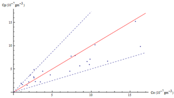 | Figure 1. Observed (Co) and predicted (Cp) scatter plot of centerline concentration using the Copenhagen dataset. Data between dotted lines correspond to ratio  |
NMSE(normalized mean square error) =  COR(correlation coefficient) =
  FS(fractional standard deviations) =
  where the subscripts
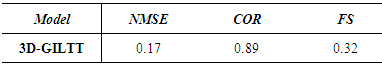
  refer to observed and predicted quantities, respectively, and the overbar indicates an averaged value. An acceptable result should reflect small values for the indices NMSE and FS and above 0.8 for the index COR. Table 2 displays the model performance evaluated by the statistical indices.
Table 2. Statistical comparison between the 3D-GILTT model and the Copenhagen dataset
 |
| |
|
A critical comment is in order here. From the data fitting point of view the ideal values of vanishing NMSE and FS are desired, whereas a correlation shall be close to unity. Recalling, that for the considered type of problem the measured phenomenon has turbulence characteristics where statistical moments beyond the first one are significant for an adequate distributional description but the underlying theoretical model considers only average values, consequently the best one may expect is a correlation from 0.8 on and above depending on the natural width and kurtosis of the measured distribution, which is not present in the deterministic model.
3. Distribution Reconstruction
As a first approach towards a procedure to recover some distributional properties from the comparison with the experimental data set, one determines the distances of each point (Co,Cp) to the ideal line, i.e. the bisector. To this end we introduce a simple change of the canonical basis 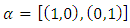 to the orthogonal base with
 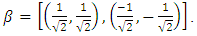 Thus, the distance from each respective point to the bisector is expressed in the new basis, by
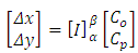 | (4) |
where  is the distance of
  to the bisector line and
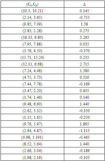
  is the matrix representing the change of basis. Table (3) shows the distance of each point resulting from the above procedure.
Table 3. Distances
 of each point (Co,Cp) to line of 45° of each point (Co,Cp) to line of 45°
 |
| |
|
Once Δ is known, one can construct a probability distribution function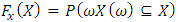 | (5) |
where  shall satisfyi) Fx (−∞) = 0,ii) Fx (∞) = 1,iii) Fx is monotonically increasing.Figure (2) shows the probability distribution function. To determine the probability density function, it is necessary to transform our discrete variable X in a continuous variable, which may be attained introducing a parametrization compatible with the restrictions for
  . The distribution profile presented in figure 2 may be parametrized by an approximation using a superposition of hyperbolic tangent functions. In the present case the implementation needed only the sum of two hyperbolic tangent functions.
 | (6) |
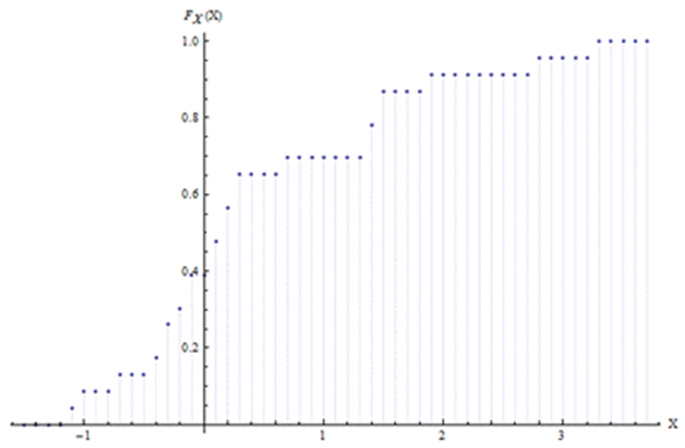 | Figure 2. Probability distribution function |
That is, FX is defined such that a1 refers to an amplitude, a2 and a4 are factors related to the growth rate of X and a3 determines translation in X for the second function.A best fit for the discrete set of data points may be obtained upon minimizing the squares of differences between the data and the parametrized probability distribution function. A variety of minimizing procedure are at hand, for simplicity we use as an optimization the method of least squares. The least squares problem is to find the parameter set a that minimizes the expression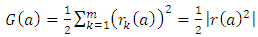 | (7) |
where a = [a1, a2, a3, a4]T and r(x) represents the difference between the data set and the proposed function, assuming m points to be adjusted to the curve.The solution of the least squares problem was implemented using Newton's method although it is known to work with local convergence only. Due to that fact a preprocessing was applied for the iterative process such that the initial values for the parameter set of the Newton iteration was within the radius of convergence.The approximation to Newton’s iterative process was established graphically and the resulting interpolation parameter set is given by a1 = 0.787834, a2 = 1.33617, a3 = 2.31281 and a4 = 1.09579. Figure (3) shows the agreement of the approximate function with the set of predicted data.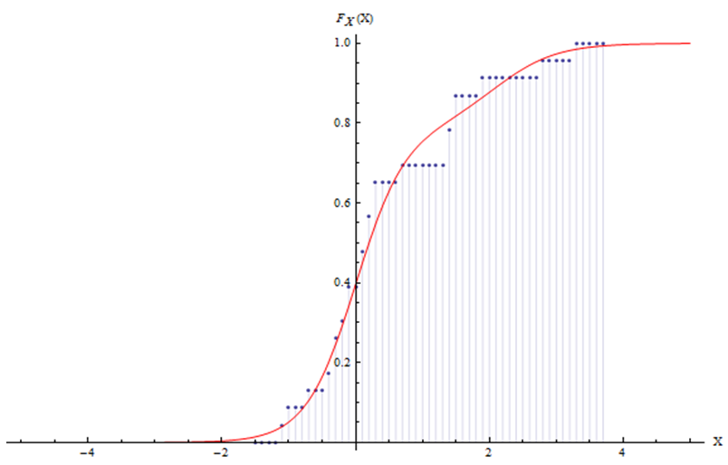 | Figure 3. Comparison of the distribution function proposed and the data points from comparison |
From these findings one can calculate the probability density function by the well known relation between the probability distribution and the probability density function,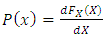 | (8) |
where  holds and further P(X) is normalized
 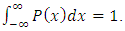 The probability density function is shown in Fig. (4). By inspection one observes a narrow peak centered at zero. If the reconstructed distribution was symmetrically around zero, one could conclude that the model describes the average values of the distribution with fairly good fidelity and the width could be used as an approximation for the second statistical moment. However, figure 2 shows also a second contribution with a maximum approaximately at X=2. This distribution which is not centered at X=0 indicates that there is either some physics missing in the model, or that there occurred errors in the measuring procedure. Without further information on data acquisition or turbulence parameterization no conclusion may be drawn so far. In any case the reconstructed distribution clearly shows the aforementioned stochastic character of the phenomenon and explains why one should expect values for COR < 1.
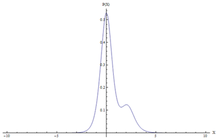 | Figure 4. Probability density function P(X) |
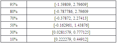
From the obtained probability density function one may obtain confidence levels for probabilities of sample data. This may be used as a further plausibility test for the reconstructed distribution. Such a procedure is necessary due to the fact that the observed data are only one sample of an unknown distribution, where the reconstructed distribution is a first estimate. The width of the distribution indicates how significant higher stochastic moments are in order to describe the turbulent phenomenon. For instance a narrow width indicates that a deterministic model is sufficient whereas a broad one indicates that a model extension is of need, i.e. additional equations for the higher statistical moments shall be proposed. The confidence level is determined by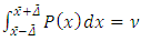 | (9) |
where  is the expectation value, i.e. the value an exact deterministic model would predict. Table 4 also shows that because of the non-centered distribution the confidence intervall is not symmetric, due to the already mentioned model or measuring errors. It is noteworthy, that the distribution width and associated confidence level is not a measure for the reliability of the model but a manifestation of the uncertainties of the turbulencde parametrization or experimental data quality.
Table 4. Confidence levels and corresponding confidence interval
 |
| |
|
4. Conclusions
The present work focussed on the pertinent question of describing the stochastic phenomenon of pollution dispersion in the planetary boundary layer by a deterministic model. Although being one of the oldest enigmas of fundamental and applied science, up to now no model exists that is able to reliably dewscribe effects of turbulent flows. Moreover, in the planetary boundary layer thermal effects are absorbed in the eddy diffusivities by their stability regime dependent parametrizations, which have their origin in the closure problem a crucial step along the derivation of the model. As a first attempt to recover the lost statistical moments by the modelling details a comparison of experimental data to the predicted values by the deterministic model was peformed. The procedure used a projection of the dispersed data points, i.e. observed versus predicted concentrations, which resulted in a discrete sample that were used to parametrize a probability distribution function. From the analysis of the obtained probability density function one could identify at least two distributions, the first one symmetric around the bisector, that corresponded to data compatible with the model and the second one that indicated or model or measurement errors. Evidently the present discussion leaves open a variety of questions, such as how to discriminate model and measurement failures, though we believe to have done a first step into a new direction.
ACKNOWLEDGEMENTS
The authors acknowledge the financial support provided by CNPq (Conselho Nacional de Desenvolvimento Científico e Tecnológico). Some of the authors thank LGSA, Tevisa and ANEEL P&D.
References
| [1] | G.A. Degrazia, D.M. Moreira, C.R.J. Campos, J.C. Carvalho, M.T. Vilhena, Comparison between an integral and algebraic formulation for the eddy diffusivity using the Copenhagen experimental dataset, Il Nuovo Cimento 25C (2002) 207–218. |
| [2] | F.H. Champagne, C.A. Friche, J.C. Larve, J.C. Wyngaard, Flux measurements flux estimation techniques, and fine scale turbulence measurements in the unstable surface layer over land, J. Atmospheric Sci. 34 (1977) 515–520. |
| [3] | G.A. Degrazia, D. Anfossi, J.C. Carvalho, C. Mangia, T. Tirabassi, Turbulence parameterization for PBL dispersion models in all stability conditions, Atmos. Environ. 34, 3575-3583, 2000. |
| [4] | G.A. Degrazia, H.F. Campos Velho, J.C. Carvalho, Nonlocal exchange coefficients for the convective boundary layer derived from spectral properties, Contrib. Atmos. Phys. 70 (1997) 57–64. |
| [5] | J. Højstrup, Velocity spectra in the unstable boundary layer, J. Atmospheric Sci. 39 (1982) 2239–2248. |
| [6] | G.A. Degrazia, C. Mangia, U. Rizza, A comparison between different methods to estimate the lateral dispersion parameter under convective conditions, J. Appl. Meteorol. 37 (1998) 227–231. |
| [7] | Vilhena, M. T., Buske, D., Degrazia, G. A., Quadros, R. S., 2011. An analytical model with temporal variable eddy diffusivity applied to contaminant dispersion in the atmospheric boundary layer. Physica A 391 (2012) 2576–2584. |
| [8] | S.E. Gryning, E. Lyck, Atmospheric dispersion from elevated source in an urban area: comparison between tracer experiments and model calculations, J. Appl. Meteorol. 23 (1984) 651–654. |
| [9] | J.S. Irwin, A theoretical variation of the wind profile power-low exponent as a function of surface roughness and stability, Atmos. Environ. 13 (1979) 191–194. |

 Abstract
 Reference
 Full-Text PDF
 Full-text HTML