1. Introduction

National as well as international initiatives are pertinent actions towards a worldwide environmental friendly politics in order to reduce increasing technological impact on terrestrial conditions. All over the world regulatory measures from international to municipal scales are established in order to reduce damage on our habitat earth. Although pioneer work in this direction is being implemented developments are far from being effective to guarantee acceptable living conditions as a countermeasure to the consequences of increasing progress in production, technological developments and many others. One key aspect related to the afore mentioned issue is pollution, where changes in the chemical composition of the planetary boundary layer of the atmosphere is one evident problem with its consequences for climate, living quality and other long term consequences.

A necessary interference in these processes shall be based on an orchestrated action where regulatory forces shall go hand in hand with scientific technological developments, especially in the question of control, planning, licensing and commissioning of installations that are the origin of pollution. It is noteworthy that by the multi-disciplinary nature of such a directive the feasibility of related actions demand for joint initiatives of the regulatory sector together with the scientific-technological academy. While latter related research establishes and characterizes fidelity of theoretical instruments such as modelling and simulation together with observational findings that focus on the identification and quantification of the pollutant components, it is the competence of the regulatory sector to implement directives, norms that are based on findings, conclusions and recommendations of the afore mentioned studies.

As a consequence of established legislation and the one to be elaborated still, the question to evaluate gravity of a pollution source and its impact on environment and society may be drawn back to the origin of pollution, i.e. the companies that are responsible for its release. In this context measurements and mathematical simulations represent complementary tools, where pollution detection is typically conducted in a limited number of locations and reproduce thus only contamination levels in these positions. Moreover, from the statistical point of view measurements are only one sample of an unknown distribution. On the other hand existing models in the literature that are being used by the scientific community are idealizations, i.e. simplifications of reality and thus are capable of reproducing only partially real scenarios. Although limited the use of these models allows to simulate the pollutant concentration in principle for any time and any localisation even where measurements are impossible to be performed. In the following we present the first step towards a synergetic structure, that shall turn models more realistic with respect to simulation of dispersion and deposition of pollutants and together with monitoring procedures open pathways to use those as a decisive instrument for legal measures. While measurements provide a reference between the model and the real scenario in the sense to validate the characteristic parameterizations of the turbulent wind field, they are restricted to localisations were measurements may be performed and those might not be the points with considerable concentrations. Legal measures based on observations only, strongly depend on the quality of choice of detection positions. Hence, comparison of observed and simulated concentrations allow within the model uncertainties to reconstruct the complete three dimensional concentration field which allows by inspection or formal analysis to identify the hotspots of the pollutant distribution. In this sense simulations also provide information for improvements of detection locations. While the insertion of modelling and simulation into a regulatory scheme is still an open question not addressed in this discussion, nevertheless the steps of modelling, measurements and optimisation are herewith an established conception.

2. Pollutant Dispersion Models

In the literature one finds besides deterministic models also stochastic approaches. Deterministic models provide as results only the mean values without further reference to higher statistical moments such as variance, skewness and kurtosis. Stochastic models contain all statistical information but need as input the turbulent regime specific probability density functions, which are in general unknown. An example for a deterministic model exhaustively discussed in the literature is represented by the advection-diffusion equation. Stochastic models are less in number and a prominent approach is by the use of the Langevin equation. Note, that for regulatory issues the awareness of the stochastic nature of the dispersion phenomenon is crucial, because from the observational point of view decisions are based on one sample only and reproduction of measurements is difficult due to permanent changes in the micro-meteorological.

2.1. A deterministic approach

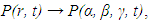
The Eulerian approach is probably most frequently used in applications for pollutant dispersion in the planetary boundary layer. A representative is the advection diffusion equation, which describes the local mean concentrations c = c(r, t) for a specific location and a specific instant (r, t) = (x, y, z, t) with one or more pollutant sources (see for example the references [1-4]).

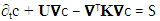(1)

Here U = (u, v, w)^T represent the vector field of mean wind velocity field, the matrix K contains the eddy diffusivities and deformations and S is a source term according to the scenario in consideration. In equation (1) the turbulent fluxes U′c′ were related to the gradient of the mean pollutant concentration weighted by the eddy diffusivity, also known as K-theory.

(2)

The simplicity of K-theory gave origin to a generalized use of this theory as a mathematical base to simulate dispersion phenomena of pollutant transport in the planetary boundary layer. However, the Fickian closure has its intrinsic limitations, it works reasonably well when the dimension of the domain in consideration where the pollutant substance is dispersed is very much larger than the largest eddy sizes involved in the diffusion process. Another crucial restriction for pollutant transport is for low concentration gradients which is incompatible with observed turbulent diffusion in the upper region of the mixed layer [5]. Despite the known limitations, the K closure is widely used for a diversity of atmospheric conditions, because it allows to effectively describe the transport by diffusion in an Eulerian fashion, which may be easily implemented in a computationally operational code.

Nevertheless, consistency of the K approach depends strongly on how turbulent diffusivity is parameterized based on the structure of the planetary boundary layer and the capacity of the model to reproduce experimental data. Hence, efforts were made to develop parameterizations for turbulence designed for practical applications in the context of air quality modeling, that mimic the essential characteristics of turbulent diffusion, but also to some extent preserve simplicity as well as flexibility of the K-theory formulation. A variety of formulations for the wind and turbulent diffusivity exist [6-10]. The objective of these procedures is to elaborate parameterizations for the turbulent diffusivity coefficients in the planetary boundary layer based on micro-meteorological parameters that may be derived from observations.

2.2. A Stochastic approach

Atmospheric turbulence and pollutant dispersion in the planetary boundary layer is a stochastic process and thus obey a stochastic law which may be expressed in form of a set of stochastic differential equations. For a time dependent regime one may assume that the Langevin equation describes reasonably well the processes of atmospheric turbulence and pollutant dispersion as discussed in details in the references [11-17]. In the Langevin equation [18] the temporal evolution in the turbulent velocity is implemented by a dissipative term, while the additional term may be understood as a gradient of a potential that depends on the fluctuations of the turbulent velocity and represents a mean field of the interaction of the pollutant with the environment in which it is immersed. And last not least there is a term that represents the stochastic contribution due to a continuous series of collisions of the particles.

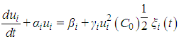Here u_i , with i = 1, 2, 3 is the Cartesian component of the turbulent velocity, which is related to the infinitesimal displacement and the wind velocity field U_i by dx_i = (U_i + u_i)dt. The coefficients α_i , β_i , γ_i of the Langevin equation depend on the pre-defined probability density function used. Here, C₀ is the Kolmogorov constant, ε is the dissipation rate of turbulent kinetic energy and ξ_i is a random increment according to the probability density function. This probability density function characterises turbulence related to the stability of the planetary boundary layer. In turbulent dispersion studies the stochastic behaviour may be classified according to stationarity or non-stationarity, depending on spatial characteristics such as homogeneity or non-homogeneity which are strongly related to the wind field, and thus are Gaussian or non-Gaussian. The most employed Lagrangian models in general consider stationary and homogeneous turbulence in the horizontal extensions but non-homogeneous in the vertical direction, depending on the stability conditions. In stable or neutral conditions the velocity distribution may be assumed as Gaussian, while in convective conditions the velocity distribution is typically non-Gaussian because of the asymmetry of the velocity distribution of the turbulent velocity field, which has its origin in the difference of the up- and downdrafts.

3. The Pollution Problem

A common problem that puts pollution dispersion problems on the agenda is growth of metropolitan areas. While the production sector is typically installed initially in peripheric areas, expansion of urban space interleaves with industrial zones and thus gives rise to the question of living condition standards where air quality is one of them. As a consequence residential neighbourhoods are exposed with polluting substances due to production processes. Federal, state and municipal laws shall guarantee protection, integrity of the environment among other related aspects. Compliance with this legislation in scientific-technical terms requires the monitoring of emission and dispersion of pollutants such as CO, CO₂, SO₂, NO_x, particulates among other substances in accordance with regulation by the respective laws.

In order to implement the procedure that combines measured data and models and to identify regions with concentrations above established limits there are two approaches, the first being a direct method and the second one has character of an inverse problem. When relevant data to determine the intensity of the emission of pollutants is provided by the pollution causing originator one is able to determine the concentration field of pollutant located far from these sources directly, upon identifying relevant meteorological parameters and specifying positions and intensity of each source involved. Data resulting from measurements in specific locations provide a consistency test between observed and simulated concentrations. In case of lacking source strength information it may become necessary to reconstruct the intensity of each pollution source that is present in the relevant region of interest starting from the specific measurements of local concentrations of the respective pollutant substances. The traditional method for this problem requires the same number of measurements as there as sources. Let C be the vector (of dimension N, number of measurements) which contains the measured concentrations in the respective positions and vector S (of size N) the unknown strength of each individual source to be determined from the known components of C. Further, the matrix T (N × N) describes in each line the attenuation of the respective source intensity from the origin along the distance to the observation point. Thus column 1 describes the contribution of the first source, column 2 of the second, and so forth. The solution of this inverse problem is given by the inversion of the equation below.

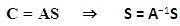(4)

This method, also known as receptor model becomes numerically ill conditioned, when for example two sources are close to each other. In this case, the inversion exists theoretically but numerically this problem has no solution, because of the fact that the determinant is quasi singular. The same problem occurs when concentration values are numerically close. From these considerations it is evident that the location of N measurements should be planned in advance (by simulations for instance) and the method to solve the inverse problem should be robust, in other words small variations should not alter significantly alter results. A method that by construction has these properties is the method of parametric inference, which moreover can be used for non-linear inverse problems. To ensure confident results, it is recommended to use twice as much points or more as there are polluting sources. Moreover, the problem turns non-linear once the matrix A depends on the source strengths and not necessarily is quadratic, i.e. of dimension N1×N2 provided N1 > N2. The formal problem to be solved is then for a given set of measured local concentrations and given the location of pollutant sources, determine the set of source intensities S_i that minimizes the following expression.

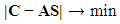(5)

The solution to this variational problem provides the best estimates for the unknowns S_i determined by the procedure sketched above (the proof of this theorem is known as theorem Cramér-Rao).

4. Optimization of Monitoring and Pollution Dispersion Analysis

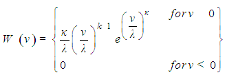
Efficient monitoring needs both measurements as well as modeling and simulating due to the fact that that each method has its limits. These aspects were already exposed in the previous section. One of the main characteristics of the present discussion consists in a complementary approach that in iterative form progressively may improve the detection configuration, which in turn allow to optimize model performance and their forecast. In the following we outline the methodology of optimizing the number of observations in different locations, as well as minimization of uncertainties in determining the intensities of the pollution sources. For a set of pollution sources it is possible to determine the field of concentrates using the solution in analytical representation discussed in detail in references [4, 2, 3, 17]. These solutions describe the field dependencies in certain instances and positions. In order to optimize the distribution of sampling position maximization of the precision of parameters to be estimated one needs the characteristics of the wind field together with the meteorological data in order to optimize predictive power. Since the wind field has variability in both modulo and direction to find the “best configuration” should take into account these probabilities describing the wind speed and direction in agreement with observational data. Let the wind speed be v = |v|, which follows a Weibull distribution W(v), where the scale and shape parameter are adjusted such as to present observation.

The directional information is obtained from the angular and speed distribution known as the wind rose diagram Ω(φ). Let the local pollutant flux be j = cv in the three dimensional domain Γ of interest and in tensor form P with a boundary surface defined by a polygon B and restrictions in the domain by ϒ. The limits restrict the geometrical area in consideration, while the restriction excludes regions within this domain where because of orographic or technical reasons it is not possible to place detector systems. 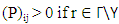and zero in the remaining coordinates. P may be used to improve the detector positioning ri using the steepest gradient such that 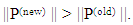The objective function E which represents the mean flux into the detector, is the one which is to be maximized locally. Upon calculating for all velocities and for all directions in agreement with the respective distribution the mean flux of the pollutant substance at position is

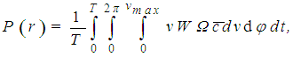where N is the number of detector systems, and T is the considered time interval. A second quantity is calculated simultaneously, ahead of each detector by adding the values of the effective flows following the line aligned with the wind direction that passes through the detectors’ centre

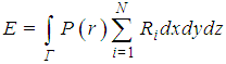
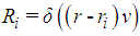Here δ signifies the Dirac delta functional. In the following the algorithm for the optimization procedure will be presented which is also the novelty of the current discussion, where validation is still a process in progress.

5. Computational Implementation

For convenience the domain is discretized in elements with edges ǫ that de- fine the resolution of the optimization problem. This means that where α, β, γ represent the three Cartesian directions.

● First initialize P_α,β,γ = 1 for all α, β, γ. Set all tensor elements outside the domain and all forbidden regions ϒ within the domain to zero

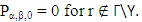● Calculate the area of feasible positions r_i and the boundary length approximated by a closed polygon B. As a first approach use the following heuristic relations. The area is proportional to the total number of detectors A ∝ N, A number NB of detectors are located on the boundary δΓ of the feasible domain. The number of detectors on the boundary N_B ∝ O(√N) (here the line integral shown below measures the length of the boundary).

Note, that in order to obtain integer numbers the floor function will be used

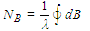● In order to place the detectors, use the dominant wind direction and place the first detector at the farest downstream edge (boundary) of the domain. Distribute with equal distances the N_B − 1 detectors on the boundary. And the rest with more or less equal distances within the domain.

● Determine P and calculate E. Determine gradients of P and displace the detectors along the gradients, where the displacement is inversely proportional to the gradient. Recalculate new area and boundaries using the polygon that describes the outer detector positions and calculate NB and N, respectively.

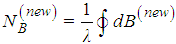and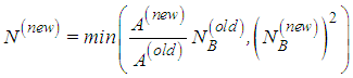

● Return to calculate P and E, until results do not change significantly.

This way the positions and the total detector number are optimised by a heuristic criterion, which should work for sufficiently convex domains. Though an additional test has to be performed reducing by hand the number of detectors and comparing the new resulting E with the previous result. Another approach could start from a small number of detectors that may be successively increased until E reaches its maximum.

6. Conclusions

The present discussion was based on an interaction between the juridical sector and the scientific technological community, which focused on the pertinent question on how to overcome barriers by profession related idiolect. Control, planning, licensing and commissioning of installations require besides the engineering aspects also juridical issues, where related actions shall work in an orchestrated fashion. In this line the present contribution showed by a conceptual analysis how mathematical simulations represent a tool that may well be incorporated into a regulatory conception in order to extend an up to now static regulatory approach by a more dynamical complement. Such a synergy could provide a framework for decision instruments and as a consequence legal measures.

As a study object we considered the pertinent problem of pollution dispersion in the planetary boundary layer, more specifically the impact on air quality and related consequences. Scientific and technical control and monitoring procedures in syntony with compliance of legislation may open pathways for in future more sustainable structures. To this end a direct and reverse engineering scenario was addressed, respectively, which may serve as a tool to identify and evaluate pollutant sources and shall improve urban planning including industrial complexes. From the presented case it is evident that theoretical approaches together with field measurements, evaluation and interpretation in juridical terms may result in effective future programs that are able to guarantee air quality in occupied spaces by humans and living beings in general.