1. Introduction

Numerical models often have difficulties for properly representing turbulent fluxes in the nocturnal boundary layer. In particular, the model performance is highly variable among different nights, and the main factor controlling this variability is the nocturnal stability regime. The stable boundary layer (SBL) has been classified in weakly stable or very stable [1, 2] or, alternatively, in terms of the coupling state between the surface and the upper levels, in coupled or decoupled [3, 4]. The weakly stable regime is characterized by continuous turbulence and generally occurs in windy nights. In this case, turbulence exists throughout the vertical extension of the SBL, characterizing a coupling between the surface and the upper boundary layer. In this case, similarity relationships are valid, and mean boundary layer variables may be predicted in a satisfactory manner by numerical models (e.g. Delage [5]; Wyngaard [6]; Duynkerke and Driedonks [7]; Cuxart et al. [8]; Steeneveld et al. [9]; among many others). On the other hand, in nights with large radiative loss and calm winds, turbulence intensity is drastically reduced by the considerably larger thermal stratification. The fluxes, in this case, are damped by the intense stability, leading to a very stable SBL regime [1, 4]. Such a regime can be related with the decoupled SBL state, when turbulence is not vertically continuous, so that the bottom part of the SBL becomes disconnected from the upper levels. The controls of the transition between the two states are not well understood, but recently van de Wiel et al. [10] and van de Wiel et al. [11] investigated the turbulence collapse in the SBL using models based on similarity and bulk relationships, and showed that such a transition tends to happens with geostrophic winds ranging from 3 to 7 m s^-1, values that are in agreement with those found by Acevedo et al. [4] using a very simple multilayer model.

The difficulty in predicting the SBL behavior under very stable conditions is associated with the fact that, in this case, often similarity relationships and stability functions lead to exceedingly small surface fluxes, causing excessive quick air cooling and subsequent unrealistically low temperatures [12, 13]. Besides, the radiative flux divergence plays an important, non-neglectable role in such regime. For this reason, building a model able to perform well in both SBL regimes constitutes a major challenge for micrometeorological research. Different turbulence formulations have been used in operational weather forecast models worldwide. Cuxart et al. [8] compared the performance of some of them in a single column model with results from Large Eddy Simulations (LES) for a idealized case of nocturnal boundary layer with continuous turbulence [14], while Svensson et al. [15] compared the performance of the same formulations for a diurnal cycle of observations during the Cooperative Atmosphere – Surface Exchange Study (CASES-99), and again the nocturnal period was continually turbulent. Steeneveld et al. [9] used a single column model coupled to a modified version of the surface scheme introduced by Duynkerke [16] to simulate the behavior of the SBL regimes for three different nights of the CASES-99 experiment: one with continuous turbulence, the second with intermittent turbulence and the third one was a radiative night. Their results indicated some limitations of the model performance in the very stable cases (the intermittent and radiative nights) and in all cases their results confirmed the importance of properly resolving the processes happening at the surface.

In this study, model outputs using four different turbulence formulations in a single column scheme are compared to observed data from eight nights, at a typically very stable site in a deforested region in Amazonia during the Large-Scale Biosphere-Atmosphere Experiment in Amazonia (LBA). The main purpose of the analysis is to provide a description of how these formulations perform in the very stable situation, which is most critical to their performance and, for this very reason, also the least studied condition. The analysis aims, therefore, at diagnosing the main problems of simulating the very stable surface layer by directly comparing model outputs to observations. The four schemes being compared differ in terms of the stability function used and on the method for representing the coupling between the surface and the atmosphere. The site and data are described in section 2. In section 3, the model, turbulence formulations and the surface scheme are described. The comparison between model results and observed data is presented and discussed in section 4. Finally, the conclusions are presented in section 5.

2. Site and Data Description

The observations used in the present analysis have been taken at a deforested site in Amazonia. Excessive long-wave radiative loss at night make very stable conditions typical there. Tethered balloon profiles of temperature, humidity and wind speed and direction have been observed there during two campaigns, in July and October 2001. In each campaign, there are 4 nights of good quality data, during which different profiles are available for each night. More detailed information on the site are provided by Sakai et al. [35], while the campaigns are described by Acevedo et al. [36].

For the period of analysis, observations of the soil temperature are available at five depths (0.14 m, 0.24 m, 0.50 m, 1.50 m and 2.00 m), while the soil heat flux was measured at two depths (0.19 m and 1.00 m) and the soil moisture content (θ) was observed at a 0.29 m depth. These data allow determining the soil thermal properties used in the present study. The local soil is a yellow latosol [35], whose median density under pasture regions in Alter do Chão Formation is ρ=1080 kg m^-3 [37]. For the entire period, the best fit for median thermal conductivity is λ=0.25 W m^-1K^-1, and the soil volumetric heat capacity (C_v) has been evaluated following de Vries [38], as C_v=(ρ/ρ_m)C_m+θC_w , where ρ_m, C_m and C_w are respectively the density and heat capacity of the mineral contents, and the water heat capacity. Asssuming that the mineral content may be approached as quartz, the values used for those quantities are: ρ_m=0.25 kg m^-3, C_m=2.13 MJ m^-3K^-1 and C_w=4.18 MJ m^-3K^-1, leading to an estimated volumetric heat capacity of the soil of C_V=1.73 MJ m^-3K^-1. Using the values of λ and C_V in equation (17), one finds the thermal capacity per area unit of the slab to be C_g=5.18×10⁵ J m^-2K^-1. As the value of the thermal conductivity is related to the volumetric heat capacity and to the apparent thermal diffusivity of the soil as λ=C_vk, the soil apparent diffusivity is k=0.144×10^-6 m² s^-1.

3. Model

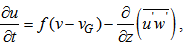
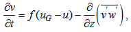
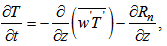
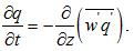
The single-column model used in the analysis consists of two parts: an atmospheric scheme and a surface scheme. The atmospheric scheme considers a horizontally homogeneous ABL, and evaluates prognostic equations for the wind components, u and v, air temperature T and specific humidity q:

(1)

(2)

(3)

(4)

In equations (1)-(4), f is the Coriolis parameter, v_G and u_G are the geostrophic wind components and R_n=ε_aσT_n⁴ is the long-wave radiative flux in the atmosphere, where σ=5.67×10^-8 W m^-2 K^-4 is the Stefan-Boltzmann constant, and ε_a is the air emissivity.

3.1. Turbulence Closure

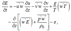
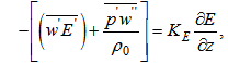
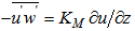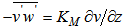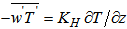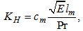
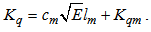
The turbulent fluxes are parameterized by K-theory as , , and 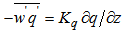. The exchange coefficients for momentum heat and humidity are K_M, K_H and K_q, respectively. They are estimated by a 1.5 turbulence closure that relates them to the TKE (E) and momentum mixing length [7, 8, 17-21]:

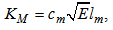(5)

(6)

(7)

In (5)-(7), c_m is an arbitrary constant whose value varies by an order of magnitude among the different turbulence formulations, as stated by Cuxart et al. [8]. Following Bélair et al. [18] the momentum mixing length is l_m=l_m,n/f_m, where l_m,n=κz is the turbulent mixing length in the neutral case (κ=0.4 is the Von Kármán constant). The mixing dependence with the stability regime is prescribed by a stability function f_m, which will be described in section 2.2. The turbulent Prandtl number Pr=K_M/K_H, for simplicity, is taken as constant and equal to 0.85 [19]. This value corresponds to the median of the range proposed by Kantha and Clayson [22, 19] for high Reynolds number flows. Following Zhang and Anthes [23], a constant K_qm that allows slow humidity diffusion, even when the turbulent mixing is completely suppressed, is used.

The turbulent exchange coefficients in equations (5)-(7) are directly dependent on the turbulence intensity, given by TKE, which is determined through its prognostic equation as:

(8)

where the two first right-hand-side (RHS) terms represent the shear production of turbulence, the third RHS term is the buoyant turbulence production/destruction, the fourth RHS term expresses the vertical transport of TKE by turbulence and pressure perturbations and the last RHS is the viscous dissipation. The transport term is parameterized as:

(9)

where K_E=K_M/σ_E, with σ_E being a constant that relates the momentum diffusion to the TKE diffusion [7, 24].

The viscous dissipation rate ε is evaluated by Kolmogorov equation [25], which considers that the turbulence is locally isotropic and homogeneous:

(10)

As the homogeneity condition is generally not applicable to the SBL, the value of c_ε varies between 0.07 and 0.7 among the different models [8]. Here, following Weng and Taylor [19], c_ε=0.164 is used in all simulations.

3.2. Mixing Length Formulations

In Equations (5)-(7), the turbulence mixing dependence on stability is given by a prescribed stability function, which depends on local scaling parameters such as the Obukhov length L or the Richardson number Ri. Such function has direct influence in the turbulent mixing under stable conditions [5, 12, 26-29]. Four different formulations are used in the present study. Two of them use the Obukhov length L as stability indicator, while the other two use the gradient Richardson number for that purpose.

3.2.1. Mixing Length Formulations that Depend on L

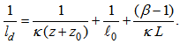
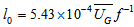
The first formulation used has been proposed by Delage [5] (hereafter DE74). In this formulation, the near-surface mixing length in neutral or stable conditions is directly proportional to κ(z+z₀), where z₀ is the roughness length, assumed as 0.1 m in the present study. The mixing length is limited by its value under neutral conditions 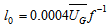, or by κLβ^-1, where β is a constant set as equal to 5. Therefore, the expression for the momentum mixing length under stable or neutral conditions is:

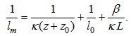(11)

DE74 also proposed a similar expression for the dissipation length scale:

(12)

The other formulation used in the present study that depends on the local value of z/L has been proposed by Degrazia et al. [29] (hereafter DG00) for stable conditions, based on Taylor statistical diffusion theory. It is important to notice that the expressions derived by DG00 are quite similar to those proposed by DE74. The mixing length depends basically on height above the ground, being limited by the neutral thermal length scale (l₀). The dependence on L indicates that the stratification has the effect of reducing the turbulent length scale, therefore increasing the molecular dissipation [29]. DG00 expression for the mixing length under neutral and stable conditions is:

(13)

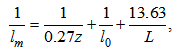
where . For simplicity, when the formulation proposed by DG00 is used in the present study, the dissipation length scale (l_d) is assumed to be equal to l_m.

3.2.2. Mixing Length Formulations that Depend on Ri

Two other mixing length formulations are considered in this study. In both of them, stability is given by the gradient Richardson number, defined as:

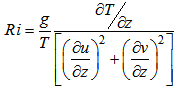(14)

The mixing length is defined as:

(15)

where l₀=κz is the mixing length under neutral thermal stratification and f_m is a stability function. When the two Ri-dependent stability functions are used, a maximum value for the neutral mixing length of l₀ = 40 m is assumed. The stability functions depends on the local Richardson number as f_m=1/(1+αRi), where α is a constant taken from observations [12, 28]. Classical SBL theory predicts that turbulent mixing is entirely suppressed by the thermal stratification when Ri exceeds a critical value, generally around 0.2 [30]. However, observations show that temporally and spatially localized turbulent activity is preserved even when Ri is supercritical. Because of that, if a formulation that follows classical theory is used and turbulence is entirely suppressed in very stable conditions, unrealistically low values of minimum temperature are usually predicted by the numerical schemes [12, 28, 30]. For this reason, the constant α in Equation (13) determines how the mixing activity decays with Ri, but always maintaining some degree of mixing activity. Two different values are considered for α in the present study. The first is α = 4.7, as proposed by Louis [12] (hereafter LO79) and the second is α = 12, following Delage [28] (hereafter DE97). In neither case turbulence is entirely suppressed at very stable conditions but, among the two, DE97 is less turbulent in that situation. Finally, in both cases, the dissipation length scale is set to be equal to the mixing length scale, that is, l_d = l_m.

3.3. Surface Scheme

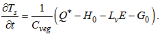
When comparing mixing length formulations in a single-column model, it is usual to prescribe the surface cooling rate for the lower boundary condition [8]. In the present study, however, besides comparing such formulations, there is also the desire of understanding the role of surface parameterization under very stable conditions. For this purpose, and considering the site features, a scheme that solves both temperatures of the soil (T_g) and of a grass layer (T_s) that covers the surface was used [7, 9, 16].

When a vegetated surface is considered, the surface temperature is evaluated through a slightly modified prognostic equation, which again considers the energy budget:

(18)

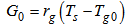C_veg is the thermal capacity of the vegetation per area unit, and G₀ is the soil heat flux at the surface, which is given by , where r_g is the heat transport conductance between the vegetation layer and the soil surface, and T_g0 is the soil temperature at the surface. As observations of C_veg and r_g are not available for the site considered, their values have been taken from the literature, from sites with similar characteristics: C_veg = 2.0×10⁴ J m^-2 K^-1 [16] and 5.0 W m^-2 K^-1 [9, 34].

To evaluate the soil temperature near the surface, an explicit scheme based on the diffusion equation has been used [9]:

(19)

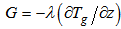where, k (m² s^-1) is the apparent soil thermal diffusivity. The soil heat flux depends directly on the temperature gradient as: . In the former equation λ is the thermal soil conductivity.

Following Duynkerke [16] and Steeneveld et al. [9], no explicit scheme for soil moisture is used here. The specific humidity at the surface is simply assumed to be the saturation specific humidity at the surface temperature.

3.4. Radiation Scheme

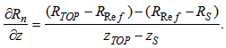
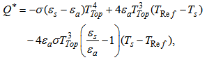
Under clear skies, Swinbank [39] parameterized the air emissivity as ε_a=9.35×10^-6 T²_Ref, where T_Ref is the air temperature at a reference height, which should be higher than the region with intense temperature gradients. According to Acevedo et al. [36], there were no major synoptic events during the nights of data collection, so that a clear sky condition is assumed. It is not necessary, therefore, to evaluate the cloud contribution to the emissivity value [34, 40]. The reference height used here was z_ref = 200 m.

The radiative flux divergence is evaluated from the long-wave emission at three different levels along the vertical domain: at the top of the domain (R_TOP= ε_aσT_TOP⁴ , z_TOP = 400 m); at the reference level, in the middle of the domain (R_Ref = ε_aσT_Ref⁴, z_Ref = 200 m); and at the first atmospheric level, just over the surface (R_S= ε_aσT_S⁴, z_S = 0.12 m) The radiative flux divergence can, therefore, be written as:

(20)

The numerator at the RHS term of Equation (20) is similar to the radiative budget at the air layers used by van de Wiel et al. [44].

Finally, following Holtslag and de Bruin [34] and van de Wiel et al. [41], the linearized surface net radiation is evaluated as:

(21)

3.5. Grid Structure and Boundary Conditions

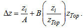
Equations (1)-(4) are discretized using finite difference equivalents, in a stretched vertical grid. The stretched scheme used here has been proposed by Degrazia et al. [42]. Some modifications, however, have been made to improve the resolution at lower levels, so that strong gradients near the surface are properly resolved, and to provide enough resolution at the upper part of the domain. The vertical increment of the vertical grid is:

(22)

where, A and B are arbitrary constants which depend on the domain height and vertical resolution desired. Here, using a 400 m high domain with 81 levels the values are A=149.4713 and B=0.0177, respectively. In this case, the three first atmospheric levels are located at 0.12 m, 0.36 m and 0.72 m, while the three higher levels are located at 371.09 m, 380.60 m and 390.24 m, respectively. The height of the vertical domain (h = 400 m) was chosen because this is the highest level where observations are available for comparison. The numerical scheme employed is a fourth order Runge-Kutta, with a 0.10 s time step. Sensitivity tests were performed, leading to the conclusion that the time step chosen is enough to warrant numerical convergence.

At the surface a non-slip condition for velocity was employed (u₀=v₀=0), and the surface temperature T_S is considered to be the vegetation temperature. Steeneveld et al. [9] showed that both T_veg and T_g0 change very fast and that, for this reason, the use of a coarse grid in the soil can lead to poor results. In this work, a 0.50 m deep homogeneous soil layer has been used, with 150 equally spaced levels. Observations show that the soil temperature at this depth was constant throughout the night and among the different nights considered, as T_gd=301.52 K. This was, therefore, the value used for substrate temperature T_m in the simulations that use the force-restore method.

At the domain top, the geostrophic wind components are u_G = 7.0 m s^-1 and v_G = 0. This value (7.0 m s^-1) was the wind speed limit beyond which the tethered balloon soundings would be halted, so that it is always a good approximation to the wind speed at the highest level of observation. Temperature and specific humidity at the domain top are taken from the observations at the first sounding of the night. While the top specific humidity is kept constant in the whole simulation, the top temperature decays due to radiative loss.

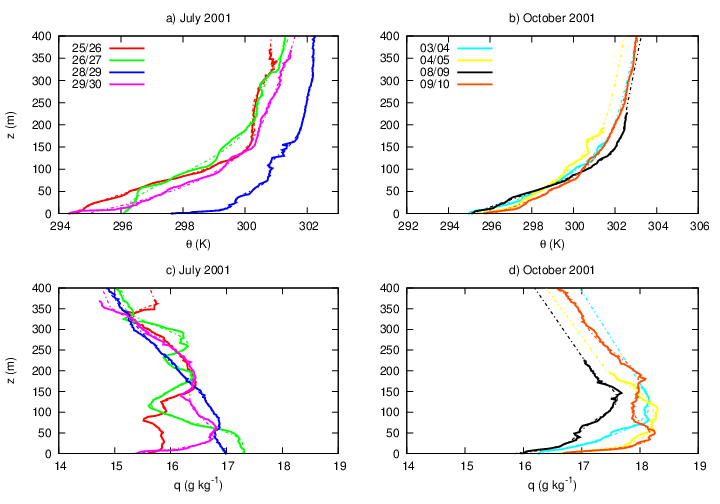Figure 1. First tethered balloon soundings of each night, indicated by the legends in the top panels. The temperatures soundings are presented in the top panels, July campaign in Figure 1(a) and October campaign is presented in Figure 1(b). The sounds for humidity are presented in bottom panels, Figure 1(c) has the soundings for July campaign, while Figure 1(d) presents the soundings of October campaign. First sounding of each night presented in Figure 1 were collected at: 25/26 July: 0033 LST; 26/27 July: 2134 LST; 28/29 July: 2130 LST; 29/30 July: 0125 LST; 03/04 October: 2151 LST; 04/05 October: 2224 LST; 08/09 October: 2151 LST; 09/10 October: 2114 LST. In all panels the each dashed line represents the initial conditions used in the simulation of the respective night

As no information about the vertical profiles of TKE exists, its initial profile was taken as in Cuxart et al. [8], i.e., the initial value of TKE at the surface is considered to be E(z₁,t₀) = 0.4 m^-2 s^-2, decaying with height as E(z₁,t₀) = 0.4(1+z_i/250)³. In all simulations a background value for TKE is used and set to be equal to E_min = 10^-9 m^-2 s^-2. For all levels, the initial value of is set to be 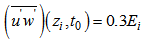while all the other fluxes are assumed to be null at the start of the simulations.

The initial conditions for temperature and specific humidity are taken from the first observation of each night, as shown in Figure 1 (solid lines). The initial values of both T(z_i,t₀) and q(z_i,t₀), have been obtained through a polynomial interpolation of the real data (dashed lines). For cases whose data do not reach the domain top, the function was just extrapolated up to the top (e.g. nights of 03/04 October 2001, 04/05 October 2001 and 08/09 October 2001, in Figures 1(b) and 1(d)).

The initial value of the meridional wind component is set to be v(z_i,t₀) = v_G = 0, while the zonal component follows the function u(z_i ≤ 100 m, t=0) = u_G-u_G(1-z_i/100), and for the remaining of the domain u = u_G. The initial profile for the wind components was an arbitrary choice, as it was not possible to determine them from the observed data as it was done for temperature and humidity.

4. Results and Discussion

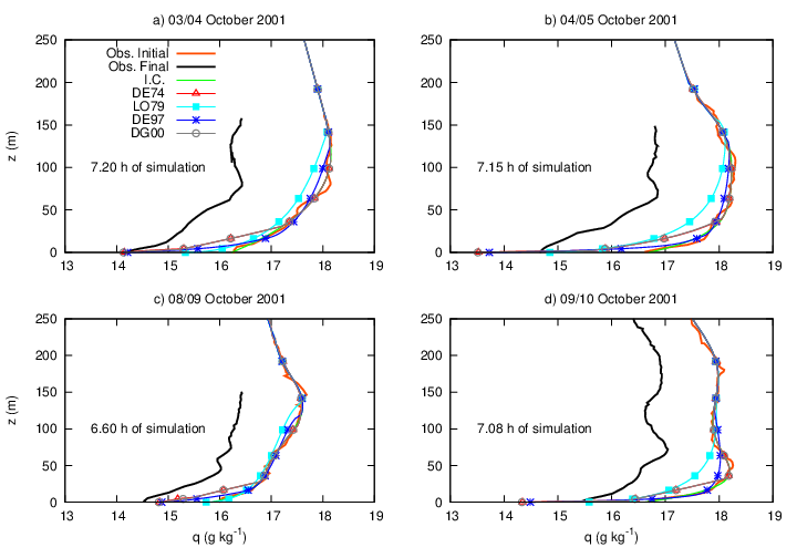
For the comparison of the stability functions, the model described in the previous section was used to simulate the temporal evolution of temperature and specific humidity profiles along the eight nights described in section 2.

Figure 2 shows the temporal evolution of temperature in different atmospheric levels, for all formulations, in a specific night. Near the surface, at 1.2 m, the behaviour using LO79 stability function differs from the others since the start of the simulation (Figure 2(a)). After a slight warming, turbulent mixing increases and causes an almost constant temperature decrease along the night (from 2130 LST). However, the surface energy loss is not enough to provide the observed surface cooling rate. When formulation DE97 is used, results are similar, but the subtle temperature increase is smaller than in the previous case and occurs after 2 hours of simulation time (2314 LST). It is also observed that after such initial increase, a constant temperature decrease happens during the last hours of the simulations. When DE97 is used, the radiative term leads to colder temperatures than when the formulation LO79 is applied. Such a difference can reach almost 0.5 K by the end of the night. When formulations that depend on the Obukhov length are considered (DE74 and DG00), temperature decreases almost uniformly along the simulation, until around 0030 LST, when a rapid temperature drop occurs, first in the DE74 formulation, and then, after a short time, also when the formulation DG00 is used. However, both cases remain slightly warmer than in the DE74 case. The sudden temperature decrease in the middle of the simulations is caused by a wind speed increase (figure not shown). Such intense wind intermittent events have been reported in the real SBL [43, 44] and also in numerical solutions using simple SBL schemes [45]. Besides the distinction between turbulence formulations near the surface, the results at the upper levels are also improved (Figures 2 (b) – 2(d)), so that temperatures in all cases (Figures not shown) are closer to the observations. Such improvement is not caused by the better performance of the turbulence formulations when the vegetation is considered, but, rather, by the better performance of the radiation scheme in this case. This result is supported by previous studies, such as van de Wiel et al. [41] and Steeneveld et al. [9], confirming the important role of the vegetated surface in modelling the SBL.

For all nights analysed, the mixing length formulations that depend on Ri lead to warmer temperatures near the surface, as observed in Figure 2(a). It is important to address what causes such differences. When stabilities functions LO79 e DE97 are considered, turbulence intensity is larger than when formulations that depend on the Obukov length are used (figure not shown). As the turbulent mixing increases, the air layer near the surface is warmed by the downward transport of warmer air from the upper part of the SBL. This is confirmed by the fact that in the upper levels there is a temperature decrease larger than when the formulations DE97 e DG00 are used (Figure 2(b) and 2(c)). This is most clearly observed in Figure 2(c), because at 103 m the temperature gradients caused by the surface cooling are smaller than they are at 48 m (Figure 2(b)).

The atmospheric level located at 250 m is above the SBL top, and at this height just the radiative flux divergence controls the temperature (Figure 2(d)).

The temperature profile evolutions for the four nights of the July campaign are shown in Figure 3. Figure 3(a), shows the performance of the turbulence formulations for the night of 25/26 July of 2001. The main differences happen near the surface, where the temperature solved by the LO79 formulation is more than 1 K warmer than those solved by the others formulations. At a time of 4.8 hours after the first sounding, the general shape of the initial temperature profile still persists, indicating that the temporal evolution of the temperature profile is basically controlled by the radiative loss. The model solutions also provide similar profile shapes, indicating that, despite its simplicity, the radiative scheme reproduces the real SBL behaviour well. Furthermore, one can notice that formulations LO79 and DE97 lead to slightly colder temperatures near the SBL top, a consequence of the stronger turbulent mixing allowed by those formulations. The initial potential temperature profile at the night of 26/27 July (Figure 3(b)) shows a less stable night than shown in Figure 3(a), and after 6.85 hours, temperature at the upper SBL is close to what was observed at that level in the initial profile, indicating a night with small radiative cooling. Model performance in this case is not good, either near the surface or in the upper SBL. The night of 28/29 July was also weakly stable at the time of the first sounding (Figure 3(c)). However, during this night, just after one hour of the first observation the surface temperature falls about 2 K (Figure not showed). This temperature decrease is not assimilated in the simulations, so that the model error increases along the night. Nevertheless, the performance of the radiative scheme is not affected by the surface temperature changes, and the model results above the SBL approach the observed temperature value. The changes observed along this night near the surface could be caused by advection of cold air, which is not prescribed or evaluated by the model. The night of 29/30 July, as the night of 25/26 July, is a night with strong stratification and the difference between the temperature near the surface and the temperature at the SBL top is almost 7 K. As discussed in the first night of this campaign, the model results near the surface and above the SBL top approach considerably to the observation, however, the last sounding of the night, 3.17 hours after the first, the temperature profile shows a cold air layer which last until 50 m, probably caused by occurrence of a local turbulent event which may lead the air just above the cold ground surface to be mixed with the warmer air present at levels above. This hypothesis could be supported by the fact that under very stable conditions, as shown in Figure 3(d), the surface becomes energetically disconnected from the upper levels of the SBL [3, 4], and weak winds tend to cool the intermediate levels of the SBL, as the turbulent mixing is restrained to the lower portion of the boundary layer. This fact is, again, not reproduced by the model. However, in this case, the model results are close to the observations, a result attributed mainly to the good performance of the radiative scheme.

Figure 4(a) shows the comparison between the results obtained after 7.2 hours of simulation with the soundings of the night of 03/04 October of 2001. Among all nights studied here, this was the worst result obtained by the model simulations. At the beginning of the night the temperature profile curvature indicates a very strong stratification, which is however, drastically reduced after 7.2 hours. This result shows that the model is not able to reproduce such a change along the night. On the other hand, for the remaining nights of the October campaign, the model estimations for the temperature profile are done satisfactorily. For 04/05 October, the model estimation at the surface is, in all formulations, around 1 K cooler than the surface observation. However, higher in the SBL, the turbulence mixture simulated by the model (clearly observed in LO79 formulation) makes the model temperature profile approach the last temperature sounding of the night (7.15h after the first observation). For 08/09 of October, the simulated temperature profiles are quite close to the observed temperature profile, even after 6.6 hours of the first sounding (Figure 4(c)). It is interesting to notice that the last sounding of the night is shallow and only shows the temperature profile within the SBL. Nevertheless, even in such a lower part of the SBL, model results are appreciably good. In most of the cases previously discussed, good performances were usually attributed to the radiative scheme. However, in this case the good performance is directly related to the model ability to correctly estimate the turbulent mixture. In spite of the night shown in Figure 4(c) being strongly stratified, the stability reduction along the night was reproduced by the model. It is clear that the LO79 formulation reaches the best result among all turbulence formulations used, and this fact shows how important it is, under very stable conditions, to maintain some turbulent activity even when the theory predicts that none should exist. The last night of October campaign (09/10 October) is presented in Figure 4(d). As in the other nights of October, the initial sounding (2114 LST) is strongly stratified. However, along the night, temperature drops more within the SBL than it does above it. The increased at lower levels is better reproduced by the formulations that use the Richardson number as a stability parameter. Again, this is a consequence of these schemes (LO79 and DE97) preserving turbulent mixing even in the most stable conditions. This inference is supported by the fact that in the most stable nights, with a sharper temperature profile, the best performance was achieved using LO79 formulation, which is the one that provides the most mixing in very stable situations. Specific humidity profiles from both campaigns also support this conclusion (Figures 6 and 7).

The model performance for specific humidity for the July campaign is presented in Figure 5. For the night of 25/26 July one can observe that after 4.8 hours of simulation the model has deviated from the initial profile only at the lowest 150 m, near the surface. The largest distinction from the initial condition, in this case, is observed for the formulations that depend on the Richardson number. At the surface, all formulations underestimate the specific humidity, and it is a consequence of the low temperatures estimated While at the surface DE74 and DG00 provided the driest values, they only deviate from the initial conditions for 30 m above the surface. At the upper atmosphere, the value of the first and last sounding are quite similar to each other.

Something similar happens for all formulations at the night of 26/27 July (Figure 5(b)). The first sounding of this night shows high values of specific humidity in the first 60 m above the surface, indicating fog. Along the night, specific humidity near the surface decreases, following temperature, as the air is saturated. The changes that occurred in the observed values of both temperature and moisture probably were caused by advection, and this fact may explain the inability of the model in forecast both quantities along the night. This result has some similarities with those obtained for the night of 28/29 July (Figure 5(c)). The first sounding of the night, as in the previous case, also shows fog (2130 LST), and moisture evolution along the night follows closely temperature variation along the night (Figure 3(c)). After the first hours, specific humidity decreases so that by the time of the last sounding (0523 LST), the specific humidity near the surface surface is almost 3 g kg^-1 drier than it was at the first observation. At the surface, the specific humidity is well predicted by all formulations. However, at upper levels, the model prediction is not good for the specific humidity. The performance for the night of 29/30 July is shown in Figure 5(d). At the time of the first sounding (0125 LST), as discussed when figure 3(d) was shown, there was a strong stratification near the surface. This stratification causes a sharp profile of specific humidity near the surface. However, along the night as the temperature decrease near the surface, specific humidity decreases in the middle portion of the SBL. As discussed before, it could be caused by a local turbulent event originated at the surface. This kind of event, that causes temperature decrease in upper atmospheric levels, also dries the atmosphere as the dry air is carried out to the upper boundary layer from the surface. As happened for temperature, no formulations were able to reproduce such a behavior, mainly due to the reduced turbulence mixing existent in such stable condition.

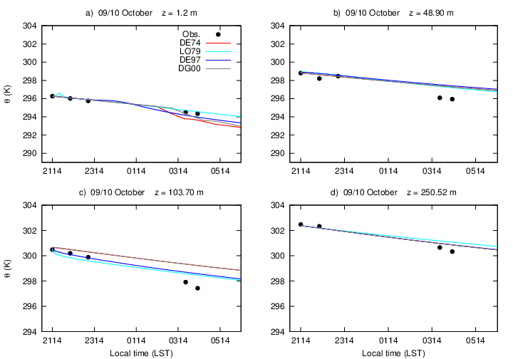Figure 2. Temporal evolution of the temperature, of the night of 09/10 October 2001, in different atmospheric levels with a surface scheme which considers a layer of vegetation of the soil. The levels in the panels are: 1.2 m (Figure 2(a)), 48.90 m (Figure 2(b)), 103.70 m (Figure2(c)) and 250.52 m (Figure 2(d)). The black dots are local temperature at the time of the sounding. The lines represent the different formulations, as indicated by the legend in top-right panel

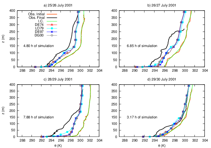Figure 3. Temperature profiles of nights of July campaign. Each night is indicated at the respective panel title. In each panel, the orange solid line is the first sounding of the night and the green dashed line is the initial condition used in the simulation. The black solid line is the last sounding of the night (soundings time are given in Table 1). Formulations performances, at the time of the last sounding of the night, are represented by the dotted lines indicated in the legend of the top-right panel

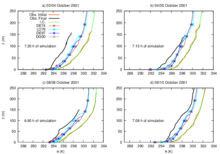Figure 4. Same as Figure 3, but, for October campaign

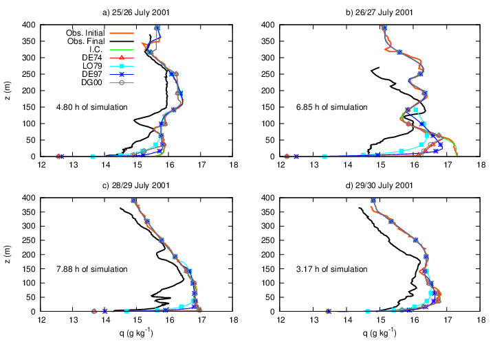Figure 5. Same as Figure 4, but, for specific humidity

The model difficulty in predicting the specific humidity profile is also observed in the nights of the October campaign (Figure 6). The evolution of the specific humidity profile, in the night of 03/04 October, is shown in figure 6(a). The initial profile shows dry air near the surface, and this feature is preserved along the night. However, humidity decreases nearly 2 g kg^-1 in the entire SBL. In spite of the formulations DE74, DE97 and DG00 forecasting the moisture value at the surface quite well, in the remaining of the domain, the value predicted was far from the observation after 7.2 hours. For the night of 04/05 October (Figure 6(b)), LO79 was the formulation that provided the best moisture prediction at the surface. However, this value is an overestimation, which also happens at higher atmospheric levels. No formulation was able to correctly predict the values of specific humidity, but, it is interesting to notice that below 50 m, the specific humidity gradient is sharper in the formulations that depend on z/L, and this has been observed in all cases analysed. This behavior indicates that those formulations have more turbulence mixing near the surface. For the night of 08/09 October (Figure 6(c)), all formulations overestimate the surface value of the specific humidity. It is probably caused by the high surface temperatures that the model estimates for this night. In figure 5(c), it was discussed that the good temperature estimation was caused by the intense turbulence activity. On the other hand, this enhanced mixing also carries the moist air to the upper levels causing a uniform overestimation by all formulations.

Figure 6. Same as Figure 5, but, for specific humidity

At night of 09/10 (Figure 6(d)), specific humidity had dropped around 1 g kg^-1, at all levels after 7.08 hours. As in the other nights of the October campaign, no turbulence formulations were able to predict such a behavior. As occurs in the temperature prediction, the specific humidity is best estimated by LO79 formulation. It shows that for nights with strong stratification it is important to consider some turbulent activity, even if the theory predicts that it should not exist. Such turbulent mixing should be included in the model due to the spatial variability of the stability, which leads to non-zero turbulent fluxes even with large values of Ri [13, 28, 46].

5. Conclusions

The comparison between model results and observed data presently being presents represents a theoretical exercise, where very important aspects, such as an advection scheme, have not taken been considered.. However, some important considerations may be inferred from the results shown.

Near the surface, all parameterizations predicted quite well the temperature evolution along the night. This result shows that the simplified surface scheme was able to reproduce correctly the energy exchange in the surface layer. For upper levels, within the SBL, the most turbulent mixing length formulations lead to solutions similar to the observations. In fact, in those cases turbulence transports the cold air from near the surface to the higher levels in the SBL, cooling them. Besides leading to colder results near the surface, formulations that suppress turbulence activity in very stable conditions are not able to couple the surface to the upper SBL [3, 4].

Two other interesting aspects of the results must be highlighted, regarding contributions from advection and radiative flux divergence in the atmosphere. In most cases it has been observed that advection must be considered when predicting profile evolution along the night, especially for humidity profiles. At the nights of 28/29 and 29/30 of July, temperature is overestimated by the model within the boundary layer, while above the SBL all formulation predictions agree with the observed profiles. It shows that, however simplified, the radiative scheme was able to reproduce the radiative cooling above the boundary layer. On the hand, humidity predictions depend solely on the turbulent scheme, and results show that in very stable conditions, such as those analysed here, a more complex scheme for humidity, which includes advection, is needed.

Finally, it is well known that it is very hard for a numerical model to reproduce the behavior of the mean variables that control the SBL flow, and that it gets harder when one tries to quantitatively reproduce observations in very stable conditions. In this way, and in agreement with previous studies [5, 12], the comparison of different mixing length formulations shows that even in the very stable case, when the Richardson exceeds its critical value, some turbulence activity must be preserved. This happens because in this situation, intermittent turbulence events are often observed, being responsible for almost all the turbulent transport [47]. Once the scheme is not able to reproduce such feature, it is necessary to always maintain some turbulent activity.

The good results with the surface and radiation schemes used here motivate to further improve the model by including an advection scheme, and by using more complete scheme for humidity. This is a task for a future work.

ACKNOWLEDGMENTS

The authors would like to thank the Brazilian agencies CAPES (Coordenação de Pessoal de Nível Superior) and CNPq (Conselho Nacional de Desenvolvimento Científico e Tecnológico) for the financial support.

List of Symbols