1. Introduction

The study of the evening transition and the stably stratified atmosphere has been investigated through field observations, theoretical analysis and numerical simulations. These studies have uncovered a number of different features of its flow pattern and some peculiar characteristics of the turbulence kinetic energy (TKE) decay under homogeneous conditions.

Considering the literature associated with field experiments we can mention: (i) the field campaigns designed to study the ABL convective decay carried out by [1] over a shallow river valley in the UK and (ii) the decay study by Acevedo and [2] using a sensor network around the Albany airport (New York), and (iii) finally the LIFTASS-2003 field campaign that was conducted over a great variety of heterogeneous surface in Germany [3].

Among the theoretical studies we can mention [4, 5] that developed a theoretical model to study the time evolution of the TKE spectrum for decaying turbulence in a convective planetary boundary layer considering the buoyancy term [4] and then incorporating the shear contribution [5]. Then Carvalho et al. [6] described the transport properties associated to decaying convective eddies in the residual layer (RL) showing that the diffusion effects associated to the decaying convective eddies strongly influence the dispersion of scalars during the sunset transition period. More recently, [7] using an analytical model to study the TKE decay in the surface layer, evidenced the role of two- transition sub-periods, each one related to the surface heat flux and characterized by a proper decaying law.

The first comprehensive numerical study of the evening TKE decay was performed by [8] NB87. Their investigation was based on the simulation with a large-eddy model (LES) considering a barotropic and horizontally homogeneous PBL in which the surface heat flux was set to zero abruptly. The reason behind NB87simulations was to investigate the turbulence decay in a non-isotropic PBL in terms of power law of time t⁻ⁿ. An important improvement of this methodology was obtained by [9] that evidenced the role of two time scales involved in this process: the convective eddy turnover time scale and an external time scale related with the daily evolution of the surface sensible heat flux. These two fundamental studies have been performed considering LES under idealized conditions (barotropic PBL and horizontal homogeneity) and for few eddy turnover times. A recent work with LES of [10] considered less idealized conditions, introducing a baroclinic geostrophic profile and an experimental surface forcing. The resulting TKE decay has been investigated until 30 eddy turnover times confirming the t^-6 scaling law for the final phase of decay as evidenced by analytical studies of [7].

Theaim of this paper is to investigate the turbulence decay in an urban area performing a Large-Eddy Simulation study under realistic environment conditions [10, 11]. In this case the setup of the LES has been implemented from remote sensing soundings and surface measurements conducted in the city of Turin (Northern Italy) under the Urban Turbulence Project (UTP) [12-14]. The LES initial profiles of temperature, specific humidity and wind components are obtained ‘‘ingesting’’ into the LES domain the corresponding vertical profiles of the same variables extracted from the experimental radio-sounding data. The surface values of potential temperature and specific humidity from Eddy Correlation measurements are used as surface forcing parameters for LES.

A further insight on the structure of turbulence during the early evening transition (EET) can be obtained from the analysis of spectral functions of the vertical wind component. This can give an indication if the spectral peak is shifted toward the largest eddies as predicted by [9] or if the position remain constant during the decay as indicated by NB87.

2. Methods

2.1. The Torino Dataset

The UTP dataset [13, 15] is composed of 15 months of continuous meteorological measurements carried out in four stations in the city of Turin (western edge of the Po Valley, Italy). In the present work we use both the UTP ground, high frequency wind measurements and the UTP wind profiler and radiometer data. The ground wind observations were collected at three levels on a mast (5, 9 and 25 m) by three sonic anemometers (two Gill Solent 1012R2 and one Gill Solent 1012R2A) on flat, grassy terrain surrounded by buildings whose distance from the measuring site is about 150 m in the north-northeast direction and about 70-90 m distance in the other directions. The potential temperature and wind profile were measured by a wind profiler and a radiometer (MTP5-HE and LAP-3000 systems respectively) of an operational station of the ARPA Piemonte meteorological network placed on a roof top (30 m) in the city centre.

2.2. The Large-Eddy Model Description and Settings

The LES code originally developed by Moeng [16] and Sullivan et al., [17] was configured in a similar way as [10]. The eddy viscosity coefficient for the momentum ν_t is given by where is the mixing length and is a velocity scale derived from the subgrid energy [18]. The boundary conditions in the horizontal were periodic, the upper boundary was specified as a rigid lid with zero mass, momentum, heat and subgrid kinetic energy fluxes, and the bottom boundary employed a no-slip condition with a prescribed roughness length (z₀). Table 1 reports the information of the extension of the grid and its resolution.

Table 1. LES setup

The velocity and temperature scales are calculated using the Monin-Obukhov (MO) Similarity Theory, that is:

(3)

where z₁ is the first vertical level of the LES grid and the similarity function are calculated using the formulation of [19].

To represent the large-scale forcing in LES the force-restore technique has been applied by using additional terms in the LES equations [10, 20].

The forcing at the surface is imposed considering the surface fluxes of temperature and moisture calculated from measured sensible (SH) and latent heat (LH) fluxes as:

(2)

In the above expressions, ρ is the density of air, C_p is the specific heat, L_v is the latent heat of vaporization and θ_v0 is the surface reference virtual temperature that is reported in Figure 1.

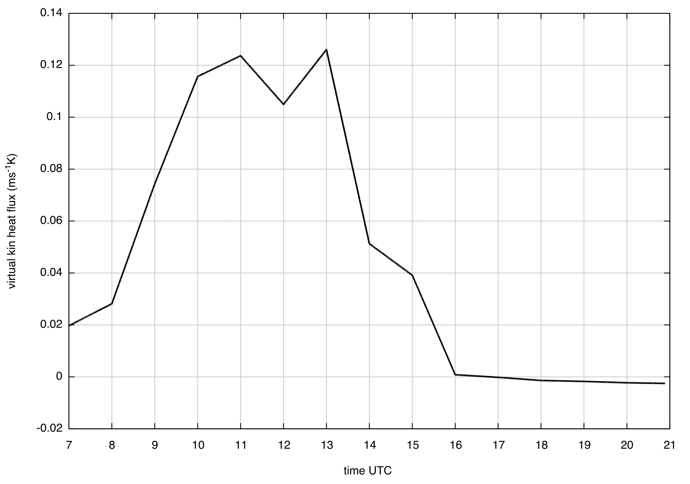Figure 1. Time series of the virtual kinematic heat flux

2.3. The Modeling of Decay

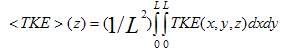
During the evening transition, the external forcing, such as the upward sensible heat flux varies very rapidly, producing a strong acceleration of the TKE decay with scaling law t^-n where n varies between -1 and -6 and t is the time since the surface heat flux reach its maximum value [7].

The turbulent mixing that is generated during the day by the unstable stratification is reduced during the night due to suppression of the vertical motion caused by the stable stratification. The evolution of the volume averaged () is a function of the two dimensionless parameters 9, and , where (in which h is the mixing height and the convective velocity scale) is the convective eddy turnover time and is the forcing time scale defined as the time period over which the surface heat flux decreases from its positive maximum value to zero [9]. Dimensional analysis suggests a power law profile of time (NB87):

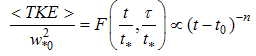(3)

where is the convective velocity scale when the sensible surface heat flux reaches its maximum value (time t₀).

Recent studies [7, 10] and past [8, 9] have revealed that the decay of energy is an accelerating process of time. In particular, during the decay period a three-stage process with the coefficient n of Eq.(3) ranging from -1 to -6 may be evidenced.

3. Results and Discussion

3.1. Surface Values

Figure 2 depicts the time series of surface friction velocity (upper panel) and the surface value of the virtual temperature (lower panel) compared with observations. It may be evidenced the reproduction of the daily cycle, and the good comparison especially during the evening hours (after 1600 UTC).

Figure 2. Time series of surface friction velocity (upper panel) and the surface value of the virtual temperature (lower panel)

Anyway, it is important to point out that the friction velocity is calculated in LES using Eq.(1) that is derived from the MO similarity theory[19] that was originally developed under the assumption of terrain homogeneity. On the other side, an urban PBL is an inherently non-linear and heterogeneous system, under permanent transition and enforced by a variety of internal and external physical process [21] that LES is not always able to reproduce.

Surface observations show again that LES data are able to reproduce the daily cycle of the virtual temperature. The LES data are obtained considering the horizontal average of the first vertical level (10.4m) while surface observations are taken with a Solent 1012R2 sonic anemometer placed at 9 m [12].

3.2. Mean Profiles

The development of the vertical structure of the Urban PBL was monitored with a wind profiler and a radiometer located on a roof top (30 m) in the city centre. In Figure 3 (a-f) it is reported the LES prediction (continuous line) of the vertical profiles of wind speed magnitude (Figure 3-upper panel) and potential temperature (Figure 3- lower panel) and its comparison with wind profiler and radiometer data (dotted line). It has been taken respectively at 1100 UTC, 1400 UTC and 1800 UTC.

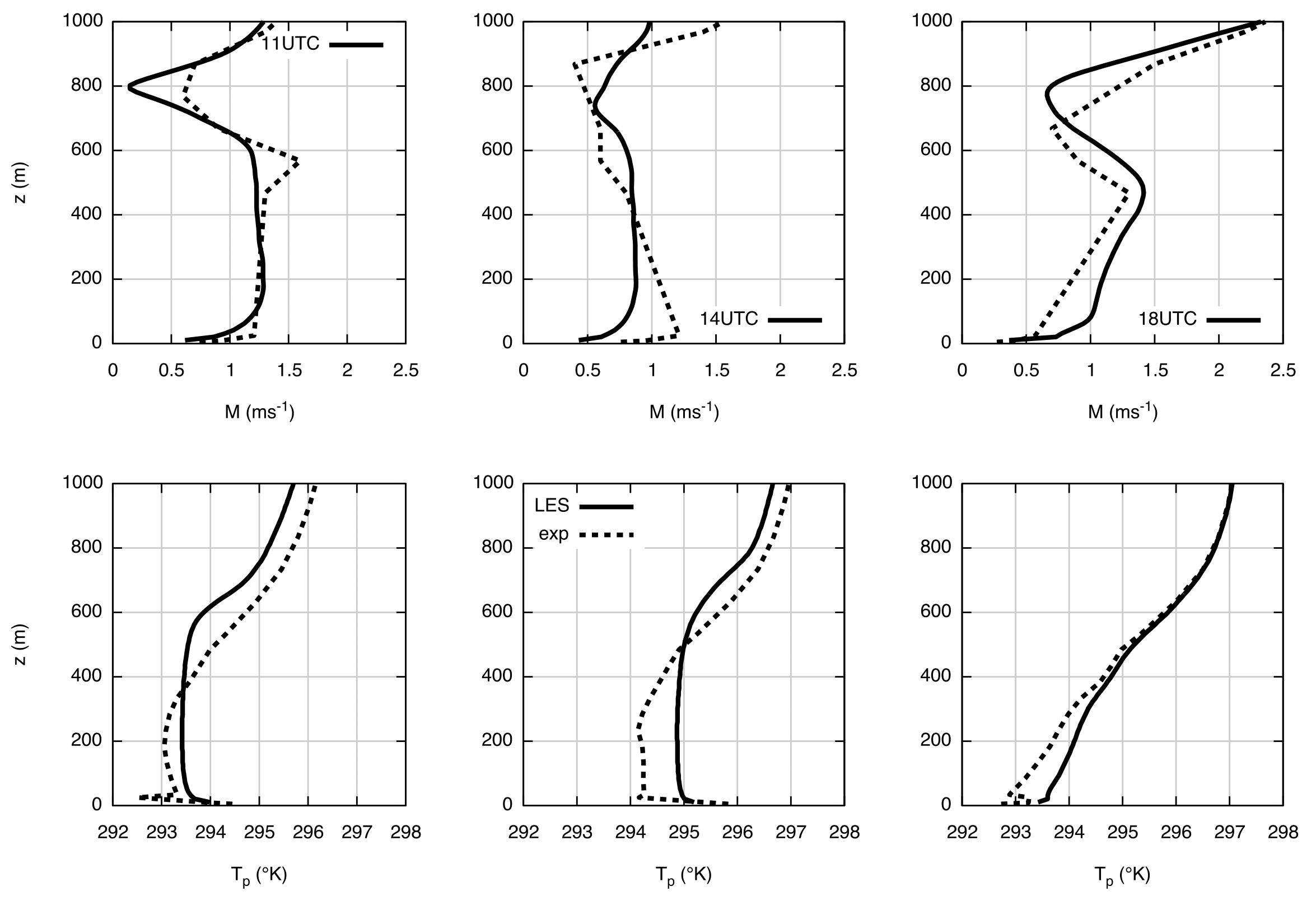Figure 3. Vertical profiles of wind speed magnitude (upper panel) and potential temperature (lower panel)

The vertical profiles of wind speed are reproduced within a reasonable range, especially at 1100 UTC and 1800UTC. It is important to point out that the value of wind speed is always lower than 1.5 ms^-1 in the interval height 0-900m. This confirms that the measurement site is characterized by low-wind-speed conditions [13, 15].

The vertical profiles of potential temperature show a good agreement between the LES results and the observed data, particularly, in the lower PBL.

3.3. Flow Visualisation

To qualitatively verify the ‘‘decay picture’’, in Figures 4 and 5 the snapshots of the vertical cross section (x–z) of vertical velocity (shaded colored scale) and the potential temperature streamlines (white lines) are shown.

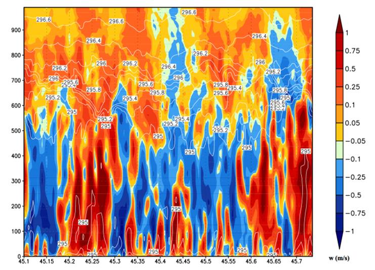Figure 4. The snapshots of the vertical cross section (x–z) of vertical velocity

Figure 4 is the snapshot taken at 1300 UTC exactly when the surface heat flux reaches its maximum value, while fig. 5 is taken at 1800Z when the surface heat flux has already reversed its sign.

At 1300UTC (Figure 4) the coherent ascending and descending structures covering a region about 600 m deep are evident and are consistent with the intense convective activity. At 1800 UTC (Figure 5), the vertical structures are absent and the temperature field is almost stably stratified.

Figure 5. The snapshots of the vertical cross section (x–z) of the potential temperature streamlines

3.4. TKE Decay and Spectra

In Figure 6 it is reported the time-height plot of the total TKE.

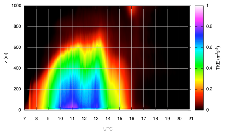Figure 6. Time-height plot of the total TKE

It is calculated following NB87 as the horizontal average:

(4)

where L is the horizontal extension of the LES domain.

Analysing Figure 6 it is evident the daily cycle that is associated with the turbulence generated by the surface heating and the low-levels wind shear. The maximum of turbulent intensity occurs between 1000 UTC and 1300 UTC in the lowest 300 m, associated with the intense downdraft/updraft structures. Figure 7 shows the boundary-layer average LES energy [] as a function of the dimensional time and defined followingNB87:

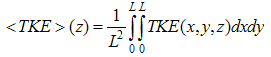(5)

where Z_eff is the boundary layer height defined as the average height of the mixing layer during TKE decay (1300-1600) UTC (Table 2). The scaling parameters that are used to nondimensionalize the TKE are defined in Table 2.

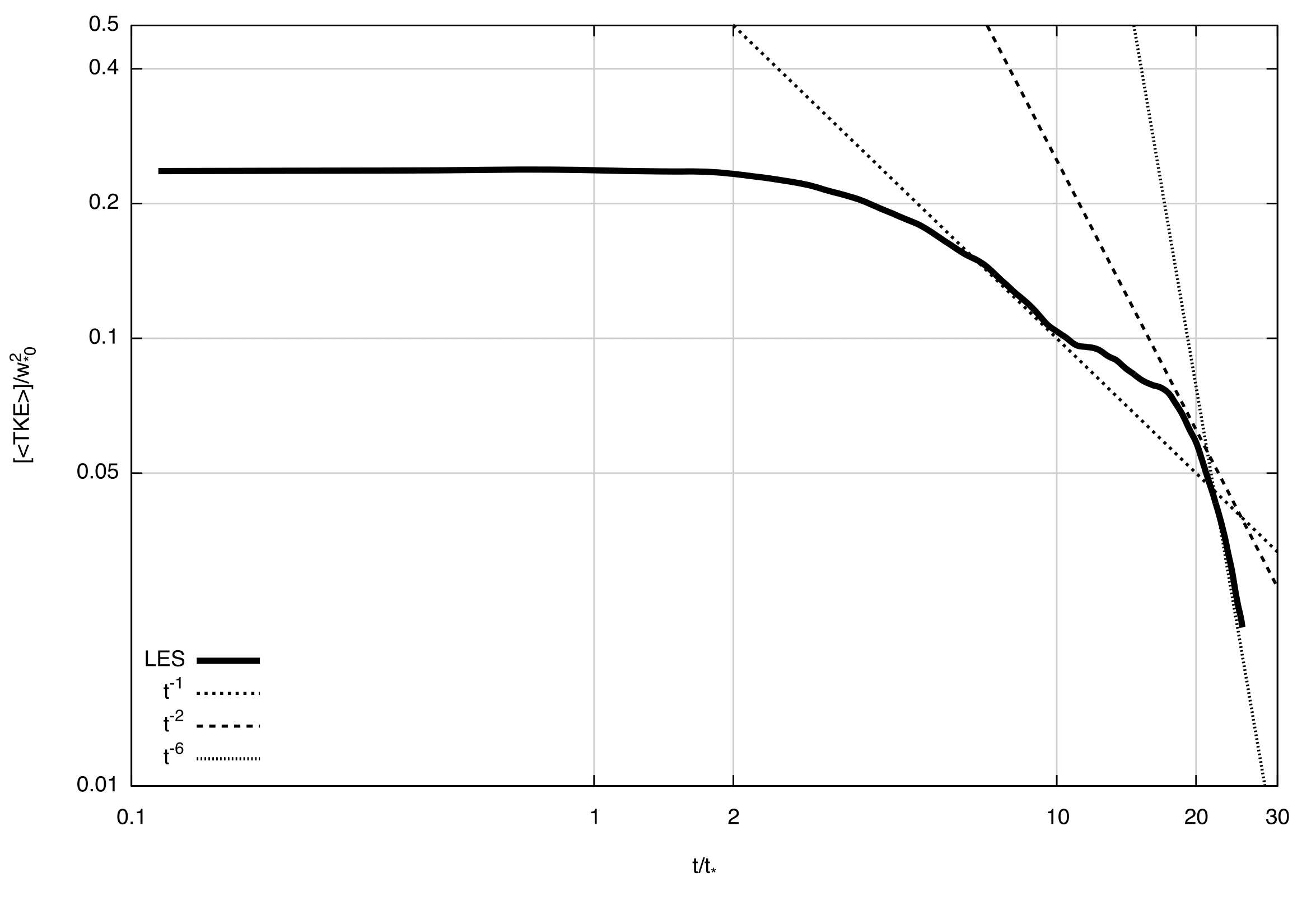Figure 7. The decay curve of []

Table 2. Meteorological parameters:       is the convective velocity at 1300UTC,       is the eddy turnover time, h the mean mixing height between 1300-1600 UTC and zeff is the vertical limit of integration

The decay curve of [] is depicted in Figure 7 jointly with the scaling curves t⁻ⁿ.

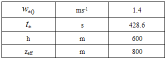
The LES results show that the t^-1 decay of [] starts after five eddy turnover time () that corresponds to 1330 UTC ending at ten turnover time or 1430 UTC. The t^-2 decay is a very rapid stage, it holds just for a short interval and finally, when the temperature stratification get stronger, the decay rate goes to the final stage characterized by a t⁻⁶ scaling law. This result verify recent findings by [7, 10], confirming that even in more complex environmental conditions, that is urban PBL and low-wind speed, the final stage of TKE decay is a t^-6 function of time.

A further understanding on the structure of turbulence during the evening transition period can be attained from the analysis of Figure 8. This figure shows the vertical velocity spectra obtained during the TKE decay. They are averaged between the ground and the height Z_eff to define a boundary-layer average vertical velocity spectra. It may be evidenced that the position of the spectral peak remain constant during the TKEdecay. This results is in agreement with the early results of NB87 which found that during the decay the spectral functions had a constant maximum value for kh~4 until .

Figure 8. The vertical velocity spectra obtained during the TKE decay

4. Conclusions

This paper presents a Large-Eddy Simulation study of the decay of the TKE during the evening transition in an urban boundary layer. To study a realistic event, LES is performed for the Urban Turbulence Project in the city of Turin (Italy).

In this context the LES simulation employed in this investigation was able to realistically reproduce the decaying PBL turbulence dynamics, including the velocity and the temperature scales at surface. The TKE decay is directly related to the solar time scale that, for the site considered here, was found to last approximately 3 h that, expressed in terms of the nondimensional eddy turnover time, is equivalent to a value close to 25.

With this work, it has been demonstrated that, during the last stage of decay the t⁻⁶ behavior persists after averaging the TKE over the entire boundary layer depth [7, 10]. This is caused by the stable stratification that causes an abrupt collapse of TKE. It is verified also that that the position of the spectral peak frequency remain constant during the TKE decay, this results is in agreement with the early findings of NB87.

ACKNOWLEDGEMENTS

Funding from the mobility program Ciência sem Fronteiras of the Brasilian government is acknowledged.