1. Introduction

The attention for offshore wind farms is increasing, since they have some unquestionable advantages with respect to onshore locations, i.e. sea wind is more intense and less turbulent than over land. For the optimal exploitation of wind resources it is of principal importance to study offshore wind conditions particularly with respect to the vertical profiles of wind and turbulence intensity.

In this context, the study of the evolution of the mean and turbulent vertical structure of the Marine Atmospheric Boundary Layer (MABL) nearby coastal offshore areas is an important subject in meteorology. The evolution of coastal MABL depends on the direction of the air flowing over it, hence on the large-scale circulation. To describe the evolution of the vertical structure of the MABL comprehensive meteorological and oceanographic observations must be carried out. Unfortunately, there are only few complete available databases due to logistics constraints together with the high costs of the offshore campaigns. Consequently, many studies have been carried out mostly from coastal locations at the shoreline or from small islands [1, 2].

In a real MABL the evolution of its vertical structure is driven by a combination of processes at different spatial-temporal scales. Astep-forward approach consists in using turbulence-resolving methodologies such as Large-Eddy Simulation (LES) coupled with a mesoscale models. In this context, LES describes physical processes at local scale and it is usually driven by the surface sensible heat flux (or surface temperature).Therefore, a crucialpoint regarding LES of the MABL is the inclusion of synoptic forcing within the LES framework. In the study of realistic MABL, one approach is to represent the large-scale forcing from atmospheric processes larger than the LES domain scale by introducing extra terms in the LES equations [3]. In this context, a recent works of [4] showed that the force-restore nudging provided an accurate simulation of the LES mean wind, temperature and humidity profiles when compared with the appropriate vertical profiles of a campaign in the Mediterranean, the LASIE (Ligurian Air-Sea Interaction Experiment) experimental [5].

The goal of this study is to implement an offshore LES with the Force-Restore nudging technique. This is realized considering offshore experimental data collected during the LASIE campaign that was performed in the Ligurian Sea during the Summer of 2007.

Two simulations are performed under different synoptic conditions. Model results have been compared against experimental soundings and mesoscale simulation. Results show that LES outperforms the mesoscale simulation, indicating that the inclusion of large-scale features into the LES model is a needed tool for providing a realistic evolution of the meteorological fields at local scale.

2. Methods

2.1. The LASIE Dataset

A comprehensive description of the LASIE campaign including the experimental setup and the observed atmospheric conditions can be found in [6]. In this paper, we consider only two days i.e.20 and 22 June 2007 with different characteristics, where the MABL has been intensively monitored using different instrumentation devices installed on different measuring platforms. Atmospheric and marine standard measurements are routinely collected by an acquisition system, at a frequency f of 0.2 Hz. Specifically: wind speed U (ms^-1) and wind direction DIR (degrees) are recorded by a bi-dimensional sonic anemometer mounted at 14.4 m height; radiation R (Wm^-2) sensors are mounted on the bulk of the structure; air temperature Ta(^oC), atmospheric pressure P(hPa) and relative humidity RH (%) are also measured, while the sea surface temperature Ts (^oC) is obtained by a temperature recorder with an extremely accurate and precise thermistor.

2.2. The Large-Eddy Model Description and Setting

The LES code of [7] and [8] is modified according to [4], to describe the Marine Atmospheric Boundary Layer (MABL) for an offshore site. It utilises the incompressible Boussinesq form of the Navier-Stokes equations considering a horizontally homogeneous boundary layer. The code solves the filtered continuity equation, the filtered momentum conservation equation written in rotational form, and the filtered heat transport equation [4]. The geostrophic wind components (U_g,V_g) are introduced as a surrogate of the horizontal gradient of the large-scale pressure fields.

The LES domain is confined around the ODAS Italia-1 spar buoy that is moored about 73 km south of Genoa. We assume homogeneous surface fluxes within the LES domain that has a horizontal extension of 5x5 km. Realistic MABL settings for LES must consider a variation of the surface heat flux that reproduces the intensity of the solar heating in offshore sites, the vertical variation of the wind, geostrophic wind profile under baroclinic conditions and the inclusion of large-scale effects. The force restore methodology provided by [9] and [4] is employed to approach the prediction of the wind, temperature and humidity profiles toward the corresponding experimental profiles from LASIE campaign. Additionally, we use the Charnock's equation [10] to characterize the sea surface roughness

Two different simulations have been performed, considering two different days from the LASIE database. Table I reports the LES settings employed for the two simulations. The horizontal domain has an extension of 5x5 km with 128² grid points. The vertical extension is 2 km with 192 grid points. The corresponding grid cell resolution is 39x39x10.5 m. The first LES run started at 1000Z (0900 LST) on 20 June, and ran for approximately 15 hours. The second run started at 0900Z (0800 LST) on 22 June and ran for 12 hours. Both runs started in correspondence with the radio-soundings launched at the ship main desk.

2.3. Description of the Two Simulated Days

Figure 1 reports the time evolution of the experimental sensible virtual heat flux (in kinematic units) for the day 20 (continuous line) and the day 22 (dotted line). It is evident for both cases the peculiar behavior for offshore sites, that is a very low value (around 10 Wm^-2) and the missing of any daily cycle that is instead a marking feature for the land counterpart. Moreover during day 22 we have oscillations between a convective MABL and a stable MABL.

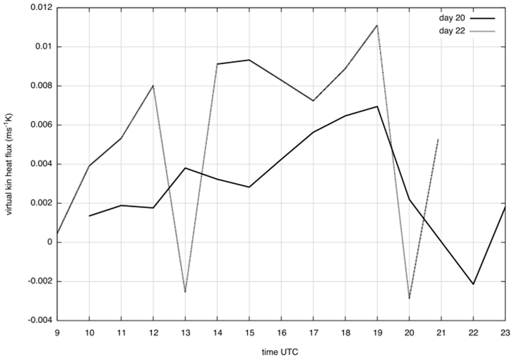Figure 1. Time evolution of the sensible heat flux for the day 20 (continuous line) and the day 22 (dotted line)

The z-time plots of the magnitude of the baroclininic geostrophic wind that is used into the LES is showed in Figure 2a (day 20) and 2b (day 22).

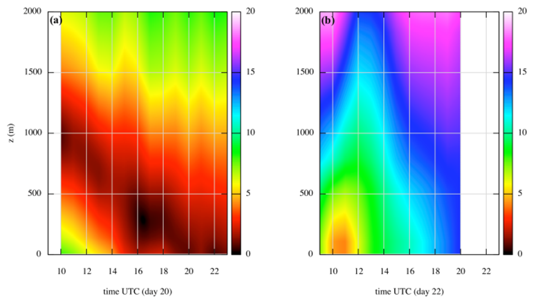Figure 2. z-time plots of the geostrophic wind magnitude for day 20 (a) and day 22 (b)

It is worth to remind that it may be seen as a surrogate of large-scale horizontal pressure gradients and thus a simple way to introduce large-scale effects into the LES-domain. It is evident the difference between day 20, that is characterized by a constant geostrophic forcing lower than 5 ms^-1 in the first 1000 meters of vertical domain, and the day 22 in which the geostrophic forcing varies with time between 5 and 15 ms^-1 in the same vertical layer. This may be an indication of different synoptic conditions during the two simulations. This is confirmed analyzing the surface wind direction measured by the sonic anemometer. Figure 3 reports the time evolution of the wind direction at sea surface for the day 20 (continuous line) and the day 22 (dotted line).

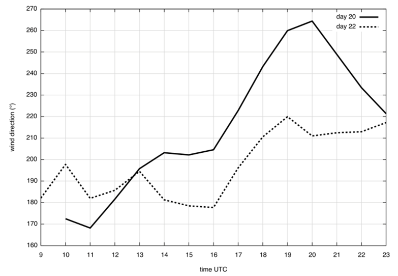Figure 3. Time evolution of the wind direction at sea surface for the day 20 (continuous line) and the day 22 (dotted line)

On the other side, [6] reported that “a weak instability occurred over the Ligurian Sea on the afternoon of 20 June, where the wind direction started to slowly rotate from offshore to onshore, both wind speed and air temperature decreased. During 21 June and 22 June a low pressure center moved towards England. The winds rotated from Southwest to South and increased in intensity”.

3. Results and Discussion

The reason of using two different atmospheric initialization corresponding to different synoptic conditions is to test the capability of LES in reproducing a variety of MABL conditions that may be controlled by the synoptic conditions.

In this context, the main issue is the assimilation of the large-scale (as compared with the size of the LES domain) variability in LES. This is accomplished in the present work implementing the force-restore nudging technique which assumes that the large-scale forcing is directly proportional to the deviation of horizontally averaged LES variables from their observed counterparts [6]. All paragraphs must be indented. All paragraphs must be justified alignment. With justified alignment, both sides of the paragraph are straight.

3.1. Surface Values and Mean Profiles for the Days 20 and 22

The Figures 4a-f show the time series of the virtual potential temperature, water vapour mixing ratio and wind speed (dotted line) for day 20 (Figure 4a,b,c) and day 22 (Figure 4d,e,f) compared with the corresponding experimental values (solid line) obtained with the sonic anemometer.

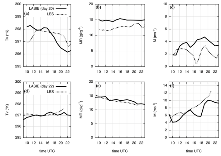Figure 4. Comparison between the surface experimental values of virtual temperature, mixing ratio and surface wind speed with the corresponding quantities calculated with LES at z1 for day 20 (a,b,c) and day 22 (d,e,f)

The simulated quantities are calculated at the first vertical point (z₁=10.4 m) of the LES grid, while the sonic anemometer are placed at 14 meters above sea level.

Figure 4a, b, c show that during the simulated period, experimental observations (solid line) indicate a small decrease (2K) of the virtual temperature (Figure 4a) a constant water vapour mixing ratio (Figure 4b) and an fluctuation of the wind speed (Figure 4c) between 2 and 5 ms^-1.

This behaviour is roughly reproduced by LES but, considering the complex situation we are simulating: wind changing direction from offshore to onshore, thus with prevailing synoptic conditions, it may be considered an encouraging comparison. It is worth to remind that the first vertical grid point of the LES grid is directly influenced by the Monin-Obukhov similarity theory that is imposed at the surface, and at the sea surface the M-O theory, some conditions, i.e. wells, might not be valid. However, this was not the case of the days of our simulation.

Figure 4d,e,f show that, during the simulated period, the experimental values of the virtual temperature (Figure 4d), water vapour mixing ratio (Figure 4e) and wind speed (Figure 4f) are in good comparison with the corresponding LES variables. This may be explained considering that the synoptic conditions, during day 22 are more toward a stable surface layer, with only a small rotation of wind direction from Southwest to South. It is important to point out that the increase of the wind is reasonable reproduced by the LES.

Figure 5a-f and 6a-f show the vertical profiles of the virtual potential temperature, water vapour mixing ratio and wind speed, respectively for day 20 (Figure 5) and day 22 (Figure 6). In each figure is reported the profiles of: radiosoundings (continuous line), LES (bold dotted line) and WRF (light dotted line). The radiosondes were launched from 2 m from the URANIA ship vessel [6], while the WRF model simulation starts at 0000 UTC on 19 June 2007 and lasts for 96 hours [6].

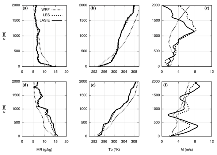Figure 5. Vertical profiles of mixing ratio (MR), potential temperature (Tp), and wind speed (M) at 1600 UTC day 20 (a,b,c) and 0000 UTC of day 21 (d,e,f)

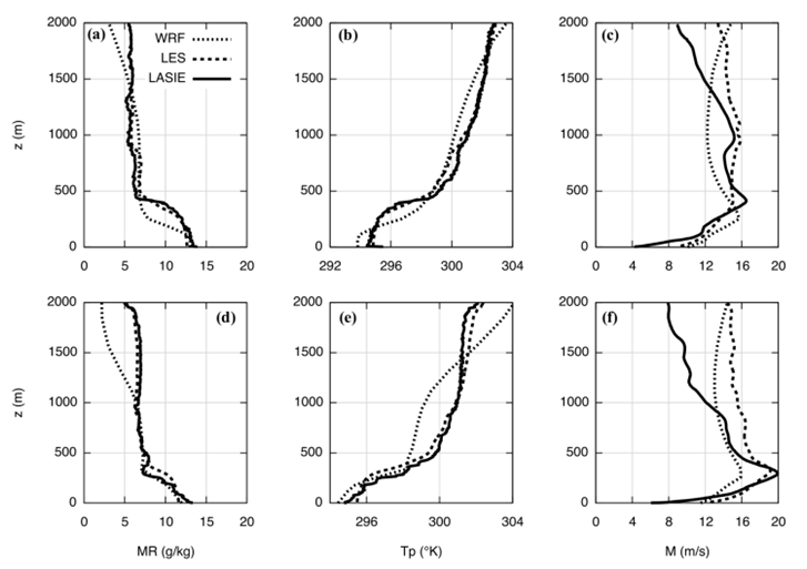Figure 6. Vertical profiles of mixing ratio (MR), potential temperature (Tp), and wind speed (M) at 1800 UTC day 22 (a,b,c) and 2100 UTC of day 22 (d,e,f)

In the upper panel of Figure 5 (a, b and c), we have reported the vertical profiles of water vapor mixing ratio (5a), the potential temperature (5b) and the magnitude of wind velocity (5c) at 1600 UTC for the 20^th of June, while in the lower panel (5d,e,f) the same quantities are depicted at time 0000 UTC for the 21^st of June.

It can be noticed a very good performance of the LES results, in particular the LES prediction of wind speed at 0000 UTC (Figure5f) seems to reproduce the formation of a low-level jet that is formed at 400 meters above sea level. This may be considered an important issue in the context of offshore wind energy. On the other side, considering the vertical profiles of mixing ratio and potential temperature, it is evident that the prediction of LES is outperforming the WRF model where the PBL physics is parameterized.

Figure 5a-f also show the fields simulated in the WRF model run, for sake of comparison, with the observed profiles and the LES run. Seemingly, although the mesoscale model is able to reproduce the general features of the observed profiles, it performs worse than the LES run. In particular, the fields are smoother and the model is not able to catch some relatively small-scale features, such as the low-level jet.

In the upper panel of Figure 6 (a, b and c), we have reported the vertical profiles of water vapour mixing ratio (6a), the potential temperature (6b) and the mean wind velocity(6c) taken at 1800 UTC of day 22, while in the lower panel (5d,e,f) the same quantities are depicted at 2100 UTC of the same day.

It is evident again the very good reproduction of the vertical profiles of mixing ratio (6a,6d) and potential temperature (6b, 6e) at both hours. Considering the mean wind speed profiles (6c,6f) the LES prediction starts to diverge from radiosoundings at 1000m at 1800 UTC, and down to 500 meters at 2100 UTC; however, the low-level jet formation is still reproduced at least in his maximum intensity.

4. Conclusions

The optimal utilisation of offshore wind resources requires the availability of long-term observation and/or numerical tools able to simulate the design of wind conditions for wind farms and wind turbines within it.

In this context, the evolution of the MABL is quite complex to monitor and simulate. The MABL is driven by an interaction of processes operating at different space/time scales, from microscale to synoptic scale, involving synoptic forcing, cloud cover, turbulence, and coastal discontinuity. All of these aspects should be properly represented in a numerical model. The approach used here includes the implementation into the LES of a horizontal large-scale pressure gradient calculated from WRF geopotential field and a force-restore nudging technique that assumes that the large-scale forcing is directly proportional to the deviation of the horizontally averaged LES variables from their observed counterparts.

The first case study considered here is characterized the by a weak instability occurred over the Ligurian Sea where the wind direction started to slowly rotate from offshore to onshore; in this case, both wind speed and air temperature decreased. The second case study is characterized by a low-pressure center that moved towards England. The winds rotated from Southwest to South and increased in intensity.

The present results indicate that the realistic evolution of the offshore surface fields and of vertical profiles require including the large-scale forcing within the LES. Moreover, both LES runs improve significantly the simulation of vertical profiles with respect to the considered mesoscale model.

Large-Eddy Simulation, even if requires a significant computational effort appears to be an encouraging technique to be applied to the simulation of offshore cases, is a promising technique that can be particularly suitable for wind energy applications.

ACKNOWLEDGEMENTS

Funding from the mobility program Ciênciasem Fronteiras of the Brasilian government is acknowledged.