1. Introduction

The main concern of a rocket launching platform is safety. This is the primary reason that platforms are built on islands, with the launchings directed to the ocean. Additional concerns include measurement of wind and gusts and scheduling launchings for those times when there are favorable weather conditions, making the work of the meteorologist among the most important during the launching process. In addition to (i) the problems that lightening can cause (electrical surges can trigger loss of control and cause destruction of rockets); (ii) the formation of fog and ice on the vehicle due the temperature and humidity fields; (iii) turbulence that can impose unacceptable stresses on key structural elements and (iv) wind that can affect the electronic guidance system, the rockets can also be affected by turbulence when positioned at the ramp, prior to the launch [1]. All these aspects make the behavior of winds and atmospheric turbulence, especially in the superficial boundary layer, to be objects of great interest in Aerospace Meteorology, because their characteristics provide basic information for both Research & Development (R&D) of rockets and analysis of the ambient conditions in the case of failed launchings, as shown by (i) Uccellini et al. [2] and Fichtl et al. [3] concerning the explosion of the Space Shuttle Challenger in 1986, (ii) Winters et al. [4] and Bellue et al. [5] regarding Columbia’s problem during its reentry flight and (iii) Kingwell et al. [6] pertaining to weather factors affecting rocket operations. Wind data are also necessary for calculation of rockets’ trajectories; for a typical Brazilian rocket launching, up to the height of 1000 m, 88% of the corrections in the trajectory are due to the wind, while above 5000 m this influence falls to 3% [7].

Concerning rocket activities, Johnson [8], for example, provides a complete compilation of the main climatic elements at the US Space Launching Centers, and Vaughan and Johnson [9] describe the lessons learned by working on aerospace meteorology during the last 50 years. Know et al. [10], using a wind tunnel, performed an experiment to study the atmospheric conditions of the island of Oenaro-Do, in order to facilitate the design of the Korean Space Center.

In Brazil, the main spaceport is located near the Atlantic ocean, at the Alcântara Space Center (ASC), on the coast of Maranhão (2° 19' S; 44° 22' W, 40 msl), 30 km from São Luiz (Fig. 1). It presents a coastal cliff with an abrupt change in roughness (from a smooth oceanic surface to a rough continental surface), associated with a topographical step of 40 m due to the cliff. The wind blowing from the ocean, initially in balance with its surface, interacts with the coastal cliff and the continental shrubbery vegetation, here with a 4 m average tree height, thus producing an Internal Boundary Layer (IBL) and its associated turbulence. The rocket launching pad (RLP) is located at 150 m from the edge of this coastal cliff (Fig. 2). So, the launchings may be significantly influenced by the local IBL. Based on this assumption the objective of the present work is to show and compare different techniques to understand the IBL flow close to the ASC.

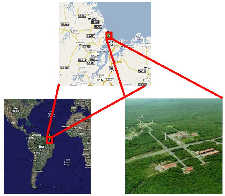Figure 1. Localization at the Alcantara Space Center (ASC)

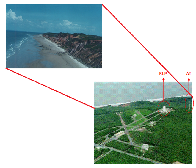Figure 2. Coastal cliff, anemometric tower (AT) and rocket launching pad (RLP) localizations at the ASC

The flow from the ocean must first surmount a cliff before it flows over the point of interest. The primary objectives here are to compare the results from the different techniques (numerical simulations, wind tunnel experiments and observational micrometeorological tower data) used to study atmospheric wind profiles and vorticity fields, as well as to quantify the height of IBL developed downwind of a coastal cliff and analyze how these parameters can affect the RLP.

2. Literature Review

A preliminary survey on the structure of the wind at the ASC, using an anemometric tower 70 m in height, with sensors for speed and wind direction at six levels, 6.0, 10.0, 16.3, 28.5, 43.0 and 70.0 m respectively, was conducted by Fisch [7], demonstrating that the winds are more intense in the dry season, with typical values between 5.0 m s^-1 at the height of 6 m and 9.0 m s^-1 at 70 m, because of the occurrence of coupling of trade winds with the movement of sea breezes. In the rainy season, in which the position of the Intertropical Convergence Zone is predominant in the characterization of the local climate, the wind in the ASC typically ranges from 3.0 m s^-1 at 6 m height to 5.0 ms^-1 at 70 m. Fisch [11], using a three-dimensional sonic anemometer, installed on a mast of 9 m localized near the RLP, in the period of August 4 through 27, 1999, characteristic of the dry season, and from April 11 through June 19, 2003, which are representative of the wet season, found that the winds are more intense in the dry season, being about 1.0 m s^-1 stronger than during the rainy season, without dependence on the stability, except for the maximum wind, which occurs in the stability-instability transition in the dry season; during the rainy season the opposite transition occurs. In 2005, Fisch [12] analyzed the behavior of the wind profile in the ASC under neutral conditions, with data collected as described in Fisch [7]. The friction velocity u_* was very peculiar, due to the seasonal variation of the wind, which is stronger in September than in March. In March u_* showed a value of 0.21 m s^-1 and in September, 0.43 m s^-1. The roughness length z₀ was between 0.66 m (March) and 0.77 m (September). The wind profiles observed ranged from 1.2 m s^-1 (level 1 of 6 m) to 2.5 m s^-1 (level 6 of 70 m) in March, and from 2.2 m s^-1 (level 1) to 4.8 m s^-1 (level 6) in September. These results were generally lower than those obtained for the ASC for these months, as shown in Fisch [7]. Data of friction velocity u_*, aerodynamic roughness length z₀, the mean velocity profiles and turbulent intensity in the ASC were also studied by Roballo and Fisch [13] and Roballo et al. [14]. In the first study, Roballo and Fisch [13] determined from observations of the anemometer tower 70 m from the ASC, that the u_* is equal to 0.32 ± 0.13 m s^-1 (rainy season) and 0.46 ± 0.11 m s^-1 (dry season), while the roughness length z₀ is equal to 0.19 ± 0.32 m (rainy season) and 0.06 ± 0.05 m (dry season). Thus the seasonality of wind profiles was demonstrated. The exponent α of the power law was also obtained for the velocity ranging from 0.19 to 0.27 over the months of the year, with correlation coefficients (R²) between 0.88 and 0.99, decreasing with height z. The validation of α with wind data from 2004 through 2005 showed that in the rainy months, estimated local velocities are greater than observed ones, perhaps due to weaker atmospheric neutrality, however, in a dry month, they were equivalent, demonstrating the neutral atmospheric conditions. In the second study Roballo et al. [14] used wind tunnel measurements with the hot wire anemometer method. The characteristics of detachment and subsequent reattachment of the flow were observed, as well the recirculation bubbles and the turbulent structure on the top of the coastal cliff. These results were shown qualitatively due to the low Reynolds number (Re) reached for the wind tunnel (10⁴ order) that did not correspond to the real atmospheric Reynolds number of the order of 10⁷.

The speed up of the flows over different geometries also has been the subject of many studies. Jackson and Hunt [15] and Britter et al. [16] analyzed the changes in the wind speed related to the size and shape of the hill and to the roughness of the surface using two-dimensional measurements in the wind tunnel and in the field and observed the increase of wind speed over the hill top. The three-dimensional experiments developed by Hunt and Snyder [17] and Hunt et al. [18] over a hill with stable and neutral stratified flow nicely showed the internal hydraulic jumps and regions of separated-flow of the structure formed around the hill in a diffusion equation analysis. In this case the recirculation zone occurs behind the hills. A similar study about the streamlines generated for stably stratified flow over a three-dimensional hill was developed by Snyder et al. [19]. Different shapes, upwind density and velocity profiles were tested to distinguish the streamlines which pass around the hill from those that pass over it, according to the Sheppard’s simple energy argument [20]. In the case of coastal cliffs the streamlines pass just over the cliff and no separation occurs. However, the influence of the coastal cliff on the flow corresponds in some respects to the well-known forward facing step (FFS) engineering paradigm. Sherry et al. [21] studied the behavior of the FFS immersed in a turbulent boundary, using water channel and wind tunnel experiments. However, the emphasis of the current paper is determining the height of the IBL, in contrast with the engineering perspective focusing on the reattachment length and the height of the recirculation region as described in Sherry’s work. Another engineering focus considers the regions of separation of the flow over the step. Pearson et al. [22] used High-speed Particle Image Velocimetry (PIV) to investigate the relationship between the upstream and downstream regions of separation in the FFS.

2.1. Internal Boundary Layer

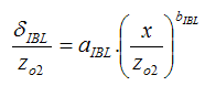
The influence of the new surface on the wind flow depends not only on its own characteristics, but also on the characteristics of the previous surface, over which the flow previously was in balance. So, a new equilibrium layer is formed (IBL), whose vertical thickness increases with the distance from the edge (Fig.3). Above this new layer the wind profile remains in balance with the previous surface, while inside it, the wind profile is adjusted to the new surface [23]. For ASC, the IBL is generated both by the surface characteristics and the presence of the coastal cliff. The thickness of the IBL may be defined as the height above ground where the wind velocity reaches a specified fraction (0.90 or 0.99) of its upstream equilibrium value [24].

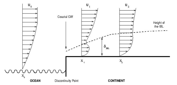Figure 3. Development of the IBL downwind of an ocean cliff and wind profiles over oceanic (x0) and continental (x1 and x2) positions

Several theoretical and experimental studies, such as Elliot [25], Pendergrass and Arya [26], Sempreviva et al. [27], Sugita and Brutsaert [28], Källstrand and Smedman [29], Jegede and Foken [30] and Savelyev and Taylor [31], especially address the problem of neutral flow over an area of change of the step roughness in a flat surface, focusing on the development of the modified wind profile, the response of the turbulent field and on the growth of the IBL. Savelyev and Taylor [31] present a table with expressions of the height of the IBL presented for 20 works starting from Elliot [25]. Non-neutral situations, considering convection, according Jegede and Foken [30], can be covered with adjustments in the neutral empirical coefficients. Subsequently attention turned to the effects of thermal stratification on the flow, growth and structure of the convective thermal IBL related to changes in temperature and heat flux at the surface [32], as shown in Batchvarova and Gryning [33] Liu et al. [34] and Hara et al. [35]. Loredo-Souza et al. [36] have suggested that for wind speeds greater than 10 ms^-1, the flow is turbulent enough to neglect thermal effects. Jackson and Hunt [15], in their studies near the surface of the hill, also affirm that although stratification has an important effect on wind, there are many instances when high winds occur and stratification has only a small effect on the flow. In work developed by Roballo and Fisch [13] it was shown that the atmospheric boundary layer at ASC can be treated as being neutral most of the time. In studies conducted at the Bolund peninsula in Denmark, Berg et al. [37] also determined that atmospheric stratification can be neglected for practical purposes, since the flow perturbations induced by changes in stability are smaller than those caused by hills.

According to a number of field and laboratory observations under neutral stability conditions, the growth of the internal boundary layer thickness (δ) follows an approximate power law, which was first proposed by Elliot [25]:

(1)

where x is the distance from the edge of the surface discontinuity, z_o2 is the downwind aerodynamic roughness length and a_IBL and b_IBL are constants that depend on the surface roughness. Empirical values for a_IBL vary from 0.35 to 0.75, and for b_IBL range from 0.1, for smooth surfaces, to 0.4, for urban areas [24]. It is worthwhile to notice that this formula may not be used for distances beyond 1-2 km from the coast, where the growth of the IBL height reaches an asymptotic value [29].

In this paper, we define δ_IBL as the height when the vertical derivative (z) of the vorticity ω becomes practically zero, which corresponds to an ω profile which is almost constant and an approximately linear variation of velocity with height, as is the case of the Planetary Boundary Layer (PBL) above the IBL.

3. Methodology

3.1. Observational Data

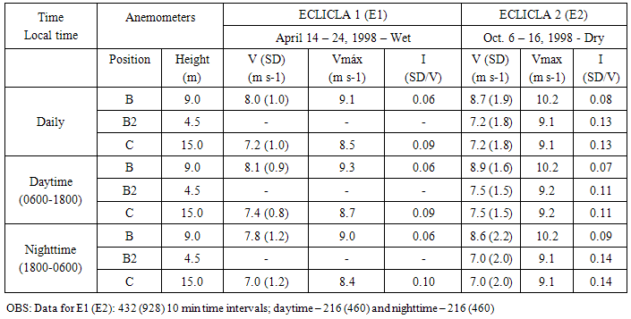
Two observational data sets were analyzed:

(i) Wind velocity and direction on a 70 m anemometric tower (AT), located 200 m downwind of the coastal cliff, measured over several years at six levels: 6.0, 10.0, 16.3, 28.5, 43.0 and 70.0 m;

(ii) The field campaigns near the edge of the cliff: ECLICLA 1 (April 14 – 24, 1998, representing the wet season) and ECLICLA 2 (October, 6-16, 1998, representing the dry season). ECLICLA is the Portuguese acronym for “Estudos da Camada Limite Interna na região do CLA” which means the study of the IBL at the ASC. The anemometers (aerovanes from R.M. Young) for both campaigns were installed on two masts on the continent downwind of the cliff: B – 50 m and C - 100 m, at the heights of 9 m and 15 m, respectively for B and C; for ECLICLA 2, an extra anemometer (B2) was added at the height of 4.5 m of the mast B (Fig. 4).

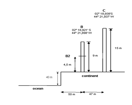Figure 4. Schematic representation of the anemometers during ECLICLA’s campaigns; in ECLICLA 2 was added the B2

3.2. Wind Tunnel Experiments

The wind tunnel (WT) experiments were made at the Prof. Kwein Lien Feng Laboratory of the Technological Institute of Aeronautics (ITA), in São José dos Campos, Brazil. This WT is an open conventional subsonic type. The test section is a square window box (465 x 465 mm2) with a length of 1200 mm. For this study, a channel apparatus with a width of 410 mm and length of 1200 mm, consisting of an uncovered wooden frame, with free edges and side walls parallel to each other and perpendicular to the floor of the wind tunnel, was used to extend the test section for the formation of the atmospheric Boundary Layer (ABL) based on the roughness correspondent to the rural terrain. Details about this simulation can be found at Pires et al. [38]. The atmospheric flow was simulated by electric fans with 30 hp (22 kW) power, which generated a maximum wind velocity of 33 m s-1. The maximum velocity actually reached was between 27 and 30 m s-1, corresponding to a Reynolds number (Re) ranging between 7.2 and 8.0 x 104 based on the height of the cliff of 40 m. In the atmosphere, the Re is basically of the order of 107 [39]. This Re was also obtained in Bolund, based on hill height and a velocity equal to 10 m s-1 [37]. For ASC, it ranged from 1.6 to 2.6 x 107, based on the height of the cliff (H) and the wind velocity (V) at the top of the boundary layer (estimated between 200 and 300 m by Pires et al [40] and approximately 300 m by Reuter et al. [41]).

Figure 5 presents the dimensions in the wind tunnel of the scaled (1:1000) cliff and the RLP, represented by a wooden block of 10 x 10 x 50 mm³, installed at the centerline. To verify the influence of the geometry of the cliff, experiments were made with inclinations of 90º, 110º and 135º. It is well- known that the direction of winds relative to the shoreline also influences the inland seabreeze and IBL [42]. So this situation was studied considering the wind flow in a perpendicular situation, as well as 45º rotations to the right and the left. The 45º angle corresponds to the dominant NE wind at ASC, as determined by Roballo and Fisch [13].

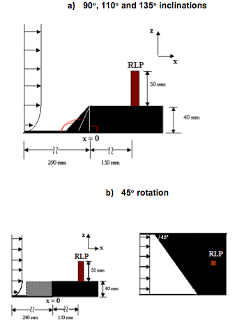Figure 5. Schematic representation of the scaled models in the wind tunnel (WT)

The atmospheric flow inside the WT was obtained using a two dimensional Particle Image Velocimetry (PIV) system [43]. The test section flow was seeded with smoke particles, approximately 5 μm in diameter, using a Rosco Fog generator. A laser Nd-YAG, 200 mJ/pulse laser of 532 nm wavelength was employed to illuminate the flow field. To image the flow field, a 60 mm diameter Nikkor lens was fitted to a 12-bits high-resolution digital camera (Dantec Dynamic HiSense 4M camera) that uses a CCD (Charge Coupled Device) with 2048 × 2048 pixels and a 7.4 μm pixel pitch. The instantaneous images were processed using the adaptive-correlation option of the commercial software developed by Dantec Dynamics (Flow Manager 4.50.17), and a 32 × 32 pixels interrogation window with 50% overlap and moving average validation was used. More information about this instrument as well as the experimental details of the measurements may be found at Pires [44].

3.3. Numerical Simulation

The Navier-Stokes equations for 2D incompressible flows, with constant density and viscosity, with velocity components u and v, respectively in the flow direction x and vertical direction z, and the vorticity component ωy, with the inclusion of the immersed boundary condition through the forcing forces Fx and Fz [45], and P being the pressure, are expressed in cartesian orthogonal coordinates as follows:

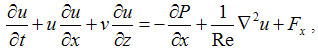(2)

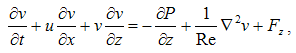(3)

together with the continuity equation:

(4)

where , t is time and Re is the Reynolds number given by .

is the height of the cliff, is the wind velocity at the top of the Oceanic Boundary Layer and is the kinematic viscosity.

Defining the vertical vorticity 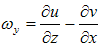, the vorticity transport equation is:

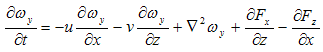(5)

From the vorticity and the continuity equations one obtains a Poisson equation for the velocity v as a function of ω_y:

(6)

The variables used are dimensionless and are related to the dimensional ones by:

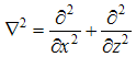
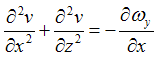
The variables with an overbar are dimensional. Although the results obtained here where stationary, the mathematical model is non stationary. The adopted code is 2D and no closure turbulence model was adopted. Future versions of the present code are expected to be able to simulate 3D flows and a subgrid model will be implemented in order to obtain a Large Eddy Simulation code.

The boundary conditions are as follows: at the inflow boundary (x = x₀), the velocity and the vorticity components are specified based on the Blasius boundary layer solution; at the outflow boundary (x = x_max), the second derivatives of the velocity and of the vorticity components in the x direction are set to zero; at the upper boundary, the derivative of v in the z direction is set to zero and the vorticity is set to decay exponentially to zero.

To investigate the IBL numerically, a technique with a high precision numerical scheme was used. It was constituted by (i) a fourth order Runge-Kutta temporal integrator with small storage and (ii) a high order compact finite differences method in the x and z directions, thus ensuring the quality of the results.

Numerical studies of flows over complex surfaces require grids and codes capable of reproducing the physics of these flows. Usually, the grid coincides with the boundaries; there are methods, however, that use orthogonal cartesian coordinates [46]. The method of immersed boundaries is one of these procedures and was introduced by Peskin [47] for incompressible flows with immersed moving bodies that exerted forces on the flow. The main advantage associated with the immersed boundaries is that the equations are solved in a rectangular domain and the fluid-solid interactions at the boundaries are modeled through an additional forcing term determined by the configuration of the boundaries.

The forcing terms used for the cliff boundary were given by:

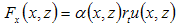(7)

where r_t is the relaxation term equal to –Re. The variable α determines the location of the immersed boundary – the coastal cliff – and is equal to 0 outside the immersed boundary, and equal to 1 inside. The transition between the two regions is expressed by a Gaussian curve. The height of the IBL is calculated by the z position, where the z-derivative of the simulated vorticity becomes nearly zero.

The computation code was developed at the Mathematical and Computational Sciences Institute (ICMC) of the University of São Paulo (USP)/ São Carlos campus and it was adapted to the coastal cliff situation [48]. The computer used was an AMD 64X2 4400 processor + with 3 Gb ram. The grid size was 305 x 801 points, with the distance between two consecutive points in the x and y direction equal dx = 7 x 10^-6 and dy = 3.5 x 10^-6, respectively. The total computational time for each simulation were between 72 and 120 hours, increasing with Reynolds number.

4. Code Validation

4.1. AT Observation and Numerical Simulation Comparison

The numeric code was validated by comparing the wind profile simulated results for a 90^o coastal cliff, with observational data collected at the anemometric tower. Figure 6 shows the observed and the simulated wind profiles for 4 cases. For Re = 2 x 10⁷ the bias (simulated minus observed wind profiles) was less than 0.7 m s^-1, and the root mean square error (rmse) ranges from 0.6 to 0.9 m s^-1. The negative bias near the surface possibly is caused by the Blasius initiation in the code, causing the velocity profile to be less turbulent. The agreement was very good, especially above a height of 10 m.

Figure 6. Observed and simulated wind profiles at x = 200 m, downwind of a 90o ocean cliff

4.2. Wind Tunnel Experiment and Numerical Simulation Comparison for Re = 7.5 x 10⁴

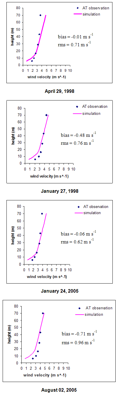
The validation was also performed through comparison with experiments in a wind tunnel. Assuming a wind velocity of 33 m s^-1, the numerical simulations and experiments were performed with Re = 7.5 x 10⁴. The heights of the IBL generated by both the WT experiment and the numerical simulation are shown on Figure 7, presenting a rmse of 1.8 m and a bias of -1.2 m, which constitutes a reasonable approximation between these results, that is, the numerical simulation represents well the behavior of the IBL formed in the WT. Only the 90º coastal cliff was considered for the validation.

Figure 7. Comparisons between wind tunnel and numerical simulation results

5. Results and Discussions

5.1. ECLICA 1 and 2

The wind characteristics during ECLICLA 1 and 2 campaigns, respectively: wind velocity (V) and its standard deviation (SD), maximum wind velocity (Vmax), and turbulent intensity (I = SD/V) are shown on Table 1.

During ECLICLA 1 The highest values of V (around 8 m s-1) occur on mast B and there is a slightly diurnal cycle: the daytime winds are stronger than in the nocturnal period, with the differences ranging from +0.3 to +0.4 ms-1. The maximum wind velocity is also stronger at mast B, which also shows lower turbulence. For the ECLICLA 2, the winds (both average and maximum) are stronger during the dry season relative to the ECLICLA 1, and they show the same pattern described earlier. The turbulent intensity (varying between 0.07 and 0.14) is stronger for all situations. The values derived from the anemometer B2 are basically the same as the ones observed by anemometer C. This is an indication that B2 and C measurements present the same characteristics, while the B measurements are different. Probably the sensor B is measuring the characteristics from the oceanic flow, while both B2 and C are representing the turbulence generated by the change of surface and the presence of the coastal cliff.

Table 1. Wind characteristics from ECLICLA 1 and 2

5.2. Wind Tunnel Experiments with Rocket Launching Pad (RLP) Model

The atmospheric flow (wind profile, streamlines and wind vorticity) obtained in wind tunnel experiments for different geometries of the coastal cliff (90º, 110º and 135º inclinations), including the presence of a RLP, are shown on Figure 8.

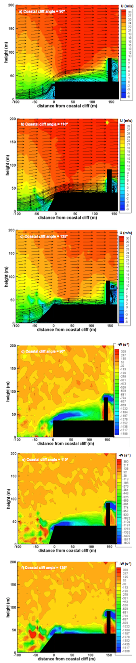Figure 8. WT wind profiles, stream lines (a,b and c) and vorticity (d, e and f) for 90º, 110º and 135º coastal cliffs and perpendicular wind direction

The geometry of the coastal cliff is a very important determinant of the flow and the turbulence. In all situations, there is the presence of a re-circulation zone. This zone is more intense (in terms of vertical depth and horizontal distance) for the 90º inclination. It is interesting to notice that the IBL depth decouples the air above from the surface. In terms of turbulence/vorticities, the 90º inclination generates high turbulence at the edge of the cliff and at the top of the RLP (located at x=150 m), which is stronger than the other 2 cases (for different geometries). The flow is not affected by the presence of RLP up to around x = 100 mm.

Figure 9 presents the wind tunnel experiments for the predominant wind direction rotated by 45º from the perpendicular flow to the coastal line. The re-circulation zone is very different from the previous case (Fig. 8). The IBL is not clearly created and it does not reach the RLP, situated at a distance of 150 m. Regarding the vorticity field, the characteristic of the recirculation bubble generated by the edge of the coastal cliff is 1600 s-1; however, the extension of the bubble decreases significantly with the incidence at sharp angles, compared to 90º, at which it is maximum.

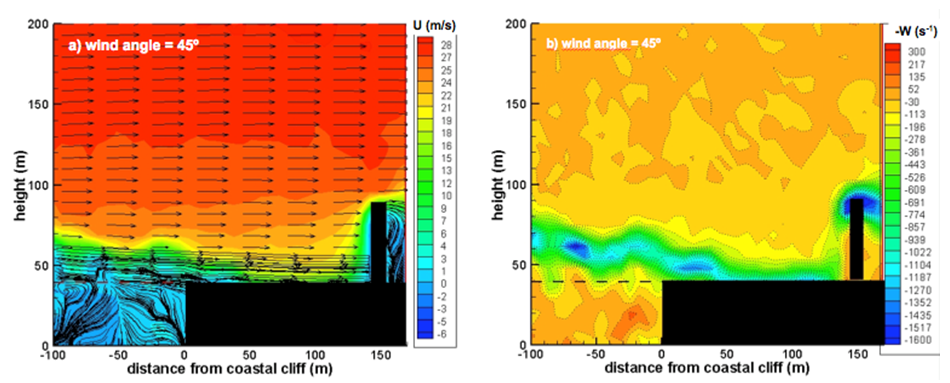Figure 9. WT wind profiles, stream lines (a) and vorticity (b) for the 45º wind direction

This is probably due to the intrinsic tridimensionality of the flow when the wind flows are other than perpendicular to the coast, causing the existence of a nonzero lateral component of the velocity.

5.3. Numerical Simulations

The vorticity field and wind profiles obtained for Re = 2.0 x 107 through the numerical simulations for all geometries (90º, 110º and 135º inclinations of the cliff) are presented in Figure 10. The maximum vorticity ranges from 4000 s-1 at the coastal cliff to 2000 s-1 at x = 150 m for all angles. The IBL demonstrated a height of 9 m at x = 0 m, 17 m at x = 50 m, 21 m at x = 100 m and 22 m at x = 150 m for the 90º inclination geometry. Making a zoom between x = 50 m and x = 100 m (Fig. 10a), it is possible to observe a profile with inverse velocity, that denotes the recirculation inside the IBL.

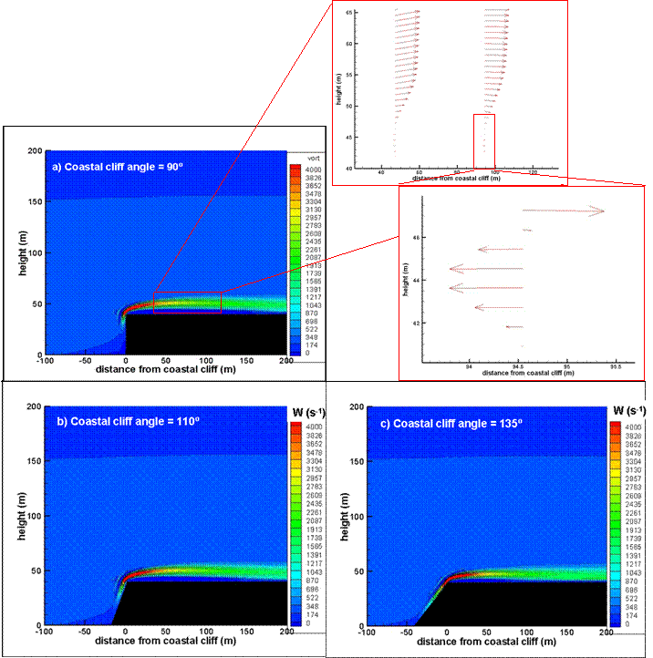Figure 10. Numerical simulation of the wind vorticity and velocity 90º, 110º and 135º coastal cliff

At the point of x = 150 m (the location of the RLP), the IBL heights were 21 m for 110º and 19 m for 135º, with a smaller recirculation and maximum vorticity around 1500 s^-1. For inclination angles smaller than 90º (not shown here but presented at Pires [44]), an increase of the IBL height, as well as the formation of a recirculation region before x = 0 are observed. For the angles 110º and 135º the recirculation region is almost nonexistent, being stronger for angles smaller than 90º. This behavior was also observed in the wind tunnel measurements (Re = 7.5 x 10⁴).

5.4. Observation, Numeric Simulation and Experiment Comparison

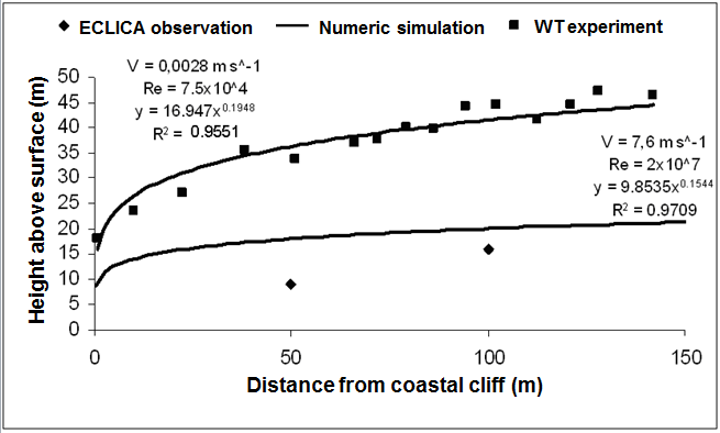
Figure 11 compares the numerical simulations (Re = 2.0 x 10⁷), the wind tunnel experiments (Re = 7.5 x 10⁴) and the ECLICLA 2 campaign results for an inclination of 90º. Also it shows their numerical expressions ax^b, with R² equal to 0.9551 and 0.9709, respectively, for the WT experiment and numeric simulation. Furthermore, adjusting the height of the WT experimental IBL with the same expression (16.95 x ^0.1948) for Re equal to 7.5 x 10⁴ resulted in R² = 0.9259 (in comparison with R² = 0.9551 for the numeric simulations).

Figure 11. Comparison between observation, experiment and numerical simulation data

For Re = 2.0 x 10⁷, as there are only two height values obtained observationally, such a comparison cannot be made, but it shows a good approximation of the heights observed during the ECLICLAs with the numerical simulation. These results, together with Figure 6, which compares wind profiles observed in the AT with the corresponding numerical simulations, demonstrate the good quality of the numerical simulations for all cases considered.

Table 2 shows the semi-empiric expressions derived by Equation 1, for different angles of the cliff. The roughness length z₀ used was 0.77 m as estimated by Fisch [12] and characteristic of the dry season at the ASC. The constant a_IBL varies from 16.1 to 47.6 for the wind tunnel experiments, and from 9.5 to 7.5 for the numerical simulation, and b_IBL is almost constant, around 0.2. The correlation coefficient (R²) is good for the WT simulations for angles 90º and 110º, but not for 135º. For numerical simulations, the R² is around 0.97 and 0.99. However, in the literature there is a wide range for reported values of a_IBL and b_IBL. Kallstrand and Smedman [29] suggest that the typical values for a_IBL are between 2 and 5, and for b_IBL stay around 0.5. According to Arya [24], the constant a_IBL varies from 0.35 and 0.75, while b_IBL varies between 0.1 and 0.4, depending on the surface.

Table 2. Values of a, b and R2 of adjusted power law IBL height

6. Conclusions and Final Comments

The analyses of the observational points (data-set from ECLICLA) show that the point B presents the greatest values of the wind velocity, which is independent of the atmospheric stability (daytime or nighttime). This is an indication that the AT, which has most of its levels above the height of mast B, is measuring the oceanic flow, as it is closer to the edge of the coastal cliff (similar to the point B mast).

The experimental test results from the wind tunnel show that the IBL can reach the RLP when the incident wind is perpendicular to the coastal cliff for all the inclination angles of the cliff. The different inclination angles of the coastal cliff do not affect the intensity of the vorticity; however, they cause alterations in the height of the IBL and influence the recirculation region: for the 90º case, the recirculation region was smaller with the lowest IBL height; for inclination angles greater than 90º, the recirculation zone remains extensive, but with a reduction in the height of the IBL.

The numerical simulations show that IBL height for the 90º and 135º cliffs present the nearest values when compared with the values determined from the ECLICLA 2 observational data for the 50 and 100 m downwind distances from the nearly vertical cliff. Considering the situation of the coastal cliff with inclination of 90º, the IBL reaches the RLP at a height of 21 m, while it is 19 m for the inclination of 135º. As the RLP is 20 m tall, it is significantly influenced by the IBL. The maximum vorticity generated on the coastal cliff of ASC is 4000 s^-1 reaching the RLP with approximately 2000 s^-1 which shows that the turbulence decreases with the distance from the edge of the cliff.

Concerning the semi-empiric expressions derived by Equation 1, the estimated values for a_IBL are greater than the ones found in the literature (between 0.35 and 0.75) which relate to cases without topographic unevenness. In this case there is the formation of a recirculation zone starting from the windward slope, probably due to the turbulence generated by the coastal cliff. Concerning to the values for b_IBL they are similar to the values found in the literature, varying between 0.1 and 0.4.

In summary, although the observational data from ECLICLA are insufficient for a deeper analysis, the wind tunnel experiment presents a good tool for the general visualization of the flow, and provides a possible approach for investigation of the influence of the wind incident inclination angles on the flow beyond the coastal cliff. However, a more representative result with this tool may be obtained through a wind tunnel that reaches greater velocities and, consequently, Reynolds numbers closer to reality (10⁷). The validation of the WT and numerical simulations with observational data from the AT showed that even a two dimensional computational model represents well the atmospheric flow at ASC, probably due to the strong surface wind, which is a combination of trade winds and the sea breeze.

ACKNOWLEDGEMENTS

LBM Pires is grateful for support received from the “Conselho Nacional de Desenvolvimento Científico e Tecnológico” (CNPq) for a doctoral fellowship (CNPq 141861/2006-1) and “Coordenacao de Aperfeicoamento de Pessoal de Nivel Superior” (CAPES) for a post-doctoral fellowship (13870-12-2). G Fisch is thankful for support from CNPq (Grants 559949/2010-3 and 303730/2010-7); LF Souza acknowledges the support of “Fundacao de Amparo a Pesquisa do Estado de Sao Paulo” (FAPESP) (process 04/16064-9). The authors would like to thank the technicians Jose Rogerio Banhara and Jose Ricardo Carvalho de Oliveira, both from the Aerodynamics Division, ALA, for their valuable help in this research.