Cláudio C. Pellegrini 1, Bardo E. J. Bodmann 2
1Depto. of Thermal and Fluid Sciences, Federal University of São João del-Rey, São João del-Rey, Brazil
2Graduate Program in Mechanical Engineering, Federal University of Rio Grande do Sul, Porto Alegre, Brazil
Correspondence to: Cláudio C. Pellegrini , Depto. of Thermal and Fluid Sciences, Federal University of São João del-Rey, São João del-Rey, Brazil.
| Email: |  |
Copyright © 2015 Scientific & Academic Publishing. All Rights Reserved.
Abstract
The present work reports on an analysis of the dynamic profile of plumes containing pollutant substances that are dispersed in the planetary boundary layer (PBL). In this line the current discussion is an attempt to describe the plume profile by its dominating physical mechanisms and its associated regions using first order perturbation theory in cylindrical coordinates. From our analysis we find that dispersion in a pollutant plume in the PBL is controlled by three physical mechanisms that compete with each other, dominating the process in different regions: advection in the centre, radial turbulence in the middle and radial diffusion at the periphery.
Keywords:
Pollutant dispersion, Atmospheric boundary layer, Perturbation techniques
Cite this paper: Cláudio C. Pellegrini , Bardo E. J. Bodmann , A Dynamic Profile of Pollutant Plumes through Perturbative Methods in Cylindrical Coordinates, American Journal of Environmental Engineering, Vol. 5 No. 1A, 2015, pp. 45-51. doi: 10.5923/s.ajee.201501.07.
1. Introduction
Air quality issues such as dispersion of pollution plumes in the planetary boundary layer (PBL) has undergone a considerable evolution from its pioneer era, due to advances in theoretical approaches based on Obukhov work combined with complete advection-diffusion models. However, the phenomenon with its complex turbulent structure is still manifest in parameterizations that hide physical details in phenomenological coefficients and it would be desirable to shade further light on at least some of involved properties. In this sense the current discussion is an attempt to describe the plume profile by its dominating physical mechanisms and its associated regions using a formulism known in the literature as first order perturbation theory. Since the plume originating from a pollutant source in a slowly varying wind field shows an approximate cylindrical symmetry along its propagation direction, we adopt cylindrical coordinates in the governing equations. The knowledge of the differential profile will them open pathways to extend the model, including in future works also thermal properties that are usually neglected due to the inherent complexity of the phenomenon. Evidently the analysis could be performed resorting to numerical methods that are, in general, more easily implemented, however suffer from severe difficulties when convergence and a mathematically sound error analysis is the subject. Differently, analytical approaches need a considerable investment when it comes to preparing the path towards solutions in analytical representation. Once such representations are found, the analysis of the solution and its dependence on physical an formal parameters is straightforward. Moreover, in the same spirit as the Gaussian solution (the first solution of the advection-diffusion equation with the wind and eddy diffusivity coefficients set constant in space), the former suggest the construction of operative analytic models. Gaussian models, so named because they are based on the Gaussian solution, are forced to represent real situations by means of empirical parameters, known as "sigmas". They are fast, simple, do not require complex meteorological input, and describe the diffusive transport in an Eulerian framework, making the use of measurements easy. For these reasons they are still widely employed for regulatory applications by environmental agencies all over the world in spite of their well-known intrinsic limits.A significant number of works regarding solutions of the advection-diffusion equation in analytical representation can be found in the literature [1-4] and references therein. All these analytical methods have in common the fact that three-dimensional, transient equations are not easy to treat. One way around this difficulty is to apply a first order perturbative analysis to the original problem before applying the transform technique. Recent meteorological literature contains a number of studies employing perturbation techniques, but none of them uses them to simplify the analysis via transform methods. In the literature some problems are obviously better suited for perturbation analysis due to the presence of a native small parameter, as is the case with the flow over smooth terrain. Regarding air pollution studies, however, very few results are found. An example is [5] that use perturbation techniques to study the transient convection-diffusion equation in Cartesian geometry. The present study uses a first order perturbation technique, known as the Intermediate Variable Technique, in cylindrical coordinates to simplify the three-dimensional advection-diffusion equation. Here we consider a inert pollutant released on a statically neutral incompressible PBL by a point source with steady or slowly varying output. We further consider that the plume is released and remains inside the surface layer. Obtained physical profiles are compared with previous results from [5].Our article is organized as follows. In section 2 we present a model analysis containing the mathematical model, the variable transformations, an order of magnitude analysis and some comments on the boundary condition dilemma. Section 3 presents a discussion on our findings and we end, in section 4, with our conclusions and future perspectives.
2. Model Analysis
2.1. The Model in Cylindrical Coordinates
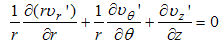
According to [6], the time-dependent three dimensional equations governing the dispersion of a passive pollutant released on a statically neutral incompressible PBL in cylindrical coordinates are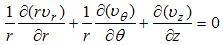 | (1) |
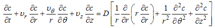 | (2) |
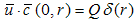
where eqn. (1) is the mass conservation equation for air and eqn. (2) for pollutant, valid in 0 < r ≤ Rp, 0 ≤ θ ≤ 2π and 0 ≤ z ≤ Lp, where Rp = Rp(z) is the plume radius and Lp is its length, defined as the distance from the source where the concentration is still measurable. We consider the case of a punctual elevated source, located at the origin of the coordinate system. In eqns. (1) and (2), symbols have their usual meaning. Thus, c is the volumetric concentration of the passive contaminant (in units of g/m3 for example), V = (υr, υθ, υz) is the wind velocity vector with cylindrical orthogonal components in the directions r, θ and z, respectively, ρ is the air density and D is the molecular diffusivity of the pollutant in the air, considered constant and invariable in all directions. If we assume plume axial symmetry, then ∂( )/ ∂θ = 0 in eqns. (1) and (2). This hypothesis is consistent with the neutral atmosphere supposition. Moreover, the boundary conditions for the problem are υr (Rp, z, t) = υr0, υz (r, Lp, t) = υz0, c (Rp, z, t) = 0, c (r, 0, t) = cs(t), c (r, Lp, t) → 0, ∂c/∂r (0, z, t) = 0. Here (υr0, υz0) is the background velocity vector and cs (t) is the concentration at the source, that is elevated a height h above the ground. The source term is absent in eqn. (2) because it is included in the boundary conditions as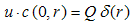 | (3) |
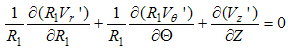
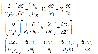
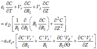
where, Q is the emission rate at the point source and δ is the Dirac-delta function. The turbulent version of eqns. (1) and (2), to the best of our knowledge, do not exist in the literature, thus we present them below. Applying the Reynolds decomposition to those equations, every dependent variable is written as a slowly varying mean part plus a rapidly varying turbulent fluctuation. Taking the time averages and supposing axial symmetry yields the new equation system. 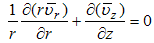 | (4) |
 | (5) |
 | (6) |
We note that in order to derive eqn. (6) the mass conservation equation multiplied by c’ was used to obtain the term in square brackets. Similar procedure may be found in standard literature to derive the turbulent Navier-Stokes equation. Here, bars over the variables represent time-averages and primes indicate turbulent fluctuations. The terms in the second pair of square brackets on the HRS of eqn. (6) are the turbulent fluxes of the contaminant. Due to the inherently tridimensional nature of turbulence, only the θ-derivatives of the mean variables were supposed to be zero in the derivation of eqn. (6). In other words, assuming axial symmetry does not imply zero tangential flux of turbulent quantities. The boundary conditions for eqn. (6) are | (7) |
 | (8) |
 | (9) |
 | (10) |
 | (11) |
 | (12) |
 | (13) |
2.2. Variable Transformations
To cast eqns. (4) to (13) into nondimensional form, typical scales for all variables shall be chosen. The physics of the problem may shed some light on this choice. We propose to use the geostrophic wind velocity, Ug, for the axial velocity because υz is expected to vary between zero at the surface and Ug at the upper bound of the PBL. Local maxima or minima may occur on the interval, but υz is not expected to attain a larger order of magnitude there. An arbitrary velocity, Vc, may be used for υr and specified later, as we shall show. We may use the concentration at the source, cs(t),, to make the mean concentration dimensionless because it is an upper bound of its value and it is expected to monotonically decrease with distance from the source. Time may be rendered dimensionless using the characteristic time interval of variations in the PBL or a characteristic time interval of variations at the source output, tc. As we shall see, the smaller of the two defines the importance of the accumulation term in eqn. (6), because it appears in the denominator of the fraction defining a small parameter in eqn. (19). We choose the interval of variations in the PBL, typically one hour, by virtue of many real sources showing a slowly varying output. The friction velocity, u* = √τs /ρ, where τs is the total stress (molecular + turbulent) at the surface is a convenient choice for scaling the turbulent velocity fluctuations. According to [7], ‘During situations where turbulence is generated or modulated near the ground, the magnitude of the surface Reynolds’ stress proves to be an important scaling variable.’ This is a well accepted idea based on the fact that the stress assumes maximum value at the surface and remains approximately constant throughout the surface layer. Indeed, a constant stress layer is often adopted [7, pg. 10] as a definition for the surface layer. The present choice for scaling the turbulent fluctuations, of course, restricts our analysis to plumes released and remaining inside the surface layer. For the turbulent concentration fluctuation we use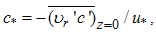 | (14) |
where  is the concentration flux at the source. The definition for was first proposed by [1] for Cartesian coordinates as
 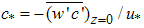 and is inspired by the definition of scaling variables as
 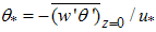 and
and 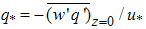 for potential temperature and moisture respectively [7]. To render the space variables dimensionless we follow [1] and recognize that the PBL and the plume have different transversal length scales. Thus, for the atmosphere we use a characteristic horizontal PBL length, L, for both r and z but, for the plume we use L for z and Rp for r. In symbols, for the air R1 = r/L and Z = z/L and for the pollutant R2 = r/Rp and Z = z/L. The space variable θ is already nondimensional and, thus θ = Θ in both cases. Using upper case letters for the dimensionless variables and the transformations indicated above, eqns. (4) to (6) become:
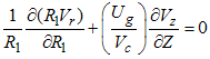 | (15) |
 | (16) |
 | (17) |
valid in 0 < R1 ≤ 1 and 0 ≤ Z ≤ 1. Here, the average bars have been omitted for simplicity and the relation R2 = R1 L/Rp implied by the previous definitions of R1 and R2 have been used. Similar expressions may be obtained for the boundary conditions. Eqn. (15) requires that Vc = O(Ug) otherwise, considering leading order only, it degenerates, thus yielding solutions that do not satisfy the boundary conditions. Substituting this relation in eqns. (15) and (17) and introducing short hand notations for the small parameters (in parenthesis) we obtain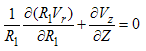 | (18) |
 | (19) |
where εt = L/Ug tc, εD = D/Ug L, ε* = u*/Ug and εc* = c*/cs. The turbulent form of the conservation of mass equation, eqn. (16) remains invariant. Typical values for the variables involved in the definitions above (see refs. [7-9]) are tc = 3,600 s, u* = 0.3 m/s and Ug = 10 m/s, D =10-5 m2/s ([8]), L = 1,000 m, Rp = 100 m, cs = O(10-7) kg/m3 and c* = O(10-8) kg/m3. The value for c* was obtained through comparison with specific humidity values, i.e., supposing that c*/ cs = O(q*/qmax), where q is the specific humidity, q* = 5•10-3 and qmax = 4•10-2. With the values listed above, the small parameters take the following typical numerical values: εt = 2.8•10-2, ε* = 3.0•10-2, εc* = 1.0•10-1, εD = 1.4•10-9. With those values it is true that εD << (ε*εc*)2, a relation that is will be used ahead.To stretch the radial coordinates, different transformations for the mass conservation equations of air and pollutant must be used again. We propose  | (20) |
for the air and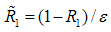 | (21) |
for the pollutant, with ε varying in the interval [0,1]. Transformations (20) and (21) reflect our expectations where to find the boundary layers in each case. For the air we assume, from our understanding of the PBL, that it is located near R1 = 0 (which means r = 0). This, of course limits our results to point sources near the ground, which is consistent with our previous hypothesis about the scaling velocities. For the pollutant, we assume the boundary layer to be at the outer boundary of the domain, at R1 = 1 (which means r = Rp). This is suggested by [11, pg. 155] based on the form of eqn. (19), specifically by the fact that the advective and molecular diffusion terms have opposite signs. The theorem presented in [11, pg. 155] applies to general linear ODEs, but here we follow the author in the hope that the idea also applies to nonlinear PDEs, specially because [1] showed in previous results using this assumption to compare well with the complete analytical solution obtained by [2] through GILTT (the Generalized Integral Laplace Transform Technique).
2.3. Order of Magnitude Analysis
Upon substituting eqns. (20) and (21) into eqn. (17) yields 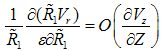 | (22) |
Substituting this order of magnitude relation and eqns. (21) and (22) into eqn. (20) yields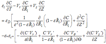 | (23) |
for  and ε in the interval [0,1], but to prevent the denominator of the second and third turbulent terms in eqn. (23) to become zero, we shall have ε of order less than one. This makes the second and third turbulent terms of order one. We also emphasize that all the advective terms have the same order of magnitude because of eqn. (22). This is a typical behaviour of boundary layers and was noticed as early as 1908, by Blasius [10] in his famous analysis of the boundary layer over a flat plate. Rewriting eqn. (22) in order of magnitude form yields:
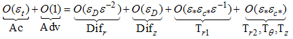 | (24) |
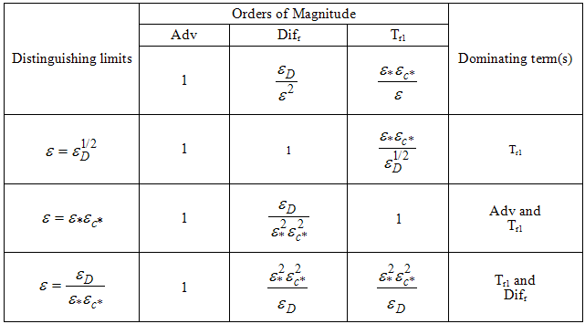
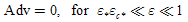
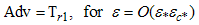
where 'Ac' stands for the accumulation term, 'Adv' for the advection term, 'Dif' for molecular diffusion and 'T' for turbulent diffusion. The subscripts in each term stand for the direction of the derivative and the numbers 1 and 2 for first and second terms in order of appearance in the equation.The values of ε for which the various terms in eqn. (24) attain the same order of magnitude are known as the distinguishing limits for the equation. They can be found by comparing all possible pairs of terms in eqn. (24). Here we need not consider all of them because some terms are always of smaller order than others as ε varies in the permissible interval (Difz and Difr, Ac and Adv, for example). Table 1 shows the result of the analysis.Table 1. Distinguishing limits – cylindrical plume
 |
| |
|
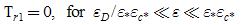
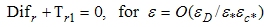
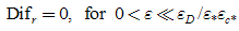
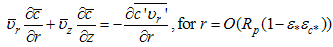
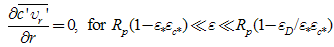
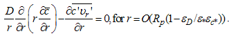
Initially, three distinguishing limits seem to result from the analysis, indicating the existence of an inner, an intermediate and an outer region on the problem, with two boundary layers. In fact, however, only two distinguishing limits exist: ε = ε*εc*, where Adv = O (Tr1), and ε = εD /ε*εc*, where Difr = O (Tr1). The value of ε where Adv = O(Difr) does not constitute a valid limit because this region is actually dominated by the Tr1 term. The previously established relation εD << (ε*εc*)2 was used to set the order relations in Table 1, as for εD /(ε*εc*)2 << 1, for example, when comparing the Adv and Tr1 terms.If we now vary ε between the two distinguishing limits, the result is the domination of only one term in eqn. (24). More specifically, in the region where εD /ε*εc* << ε << ε*εc*, only Tr1 dominates. Allowing ε to vary in the whole permissible range will lead to five approximated different first order equations. Denominating the regions from the centre outwards with one to five, the first one is dominated by advection, so that the leading order equation to be solved is eqn. (25). The subsequent region, already discussed in Table 1, has an associated equation (26), with advection and turbulence contributions. The third layer is dominated by turbulence, consequently the solution of eqn. (27) determines the leading order characteristics. The fourth layer contains beside turbulence also molecular diffusion (eqn. (28)). Last not least, the outer layer shows molecular diffusion dominance, eq. (29). Figure 1 sketches the layers of the plume with their respective leading order terms according to eqns. (25) to (29), however out of scale.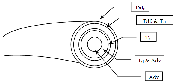 | Figure 1. Schematic drawing of the cylindrical pollutant plume, showing regions of dominance of the terms in eqn. (6) |
 | (25) |
 | (26) |
 | (27) |
 | (28) |
 | (29) |
Restoring the dimensional form of the previous equations reads: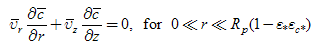 | (30) |
 | (31) |
 | (32) |
 | (33) |
 | (34) |
To return the regions of validity of eqns. (25) to (29) to dimensional form, eqn. (21) was used, noting that after the stretching transformation  shall hold.
2.4. The Boundary Condition Dilemma
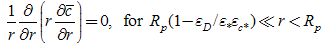
The analysis of the previous section identified five regions with distinct dynamic characteristics. While for the shell with predominant molecular-diffusion, turbulent-diffusion and advection, respectively, an analytical solution may be constructed, this is not the case for the mixed molecular and turbulent diffusion or the advection and turbulent diffusion regions. A traditional solution of the first order approximations by the Matched Asymptotic Expansion methods would require a solution for eqns. (31) and (33), which have enough structure to represent the full original equation in their regions of validity. The necessary boundary conditions for them would come from eqns. (9) and (12) and from the matching condition at the common region of validity. As mentioned before, they are still too complicated to be solved by traditional analytical methods even with a simple turbulence closure model [8] where stochastic models are replaced by relations to their respective deterministic terms. The principal dilemma comes from the fact that, to a reasonable approximation, the centre and the outer boundary conditions may be employed for the inner boundary of the advection-turbulent diffusion shell and the outer boundary for the molecular-turbulent driven region. By reasonable approximation we mean that the error is of same order of magnitude than the terms neglected by the perturbative procedure in the equation. However, the matching between the two zones two and four at their overlapping zone seems out of reach here. An attempt to circumvent this problem is sketched as follows. Solving equations other than (31) and (33) may give some information, but the process still lacks appropriate boundary conditions. To illustrate this we solve eqn. (30) by integrating it twice, resulting in an equation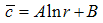 | (35) |
valid for a region very near to the plume periphery, in which A and B are unknown functions of z. Using the boundary condition expressed by eqn. (9) yields | (36) |
where A < 0, because r < Rp. Unfortunately there is no proper boundary condition available to obtain A from eqn. (36), once there is no region of common validity between eqns. (32) and (34), since the region in between is too tick to allow for overlapping. Moreover, solving eqn, (33) would yield yet another integration constant. Nevertheless, eqn. (36) could be solved in a flux-gradient approach, using a supposedly known pollutant flux at the plume periphery. A similar scheme can be used to obtain the well-known logarithmic law for a neutral surface layer over flat terrain [8] but will only work in a Cartesian coordinate system, because a simple turbulence model is necessary. Alternative trials without conclusive results so far are in progress and we consider this issue beyond the scope of the present discussion.
3. Discussion
From the previous analysis it follows that dispersion in a pollutant plume in the ABL is controlled by three physical mechanisms that compete with each other, dominating the process in different regions: advection in the centre, radial turbulence in the middle and radial diffusion at the periphery. Other mechanisms such as longitudinal diffusion and turbulence are lower order corrections to these dominant effects and can be neglected in a first order perturbation approach. The accumulation effect (positive or negative), due to time variations on the source, is only important if we suppose a rapidly varying source output, which is not an issue in the present discussion.The perturbation approach also shows that the three competing physical mechanisms balance each other in pairs, creating a typical two boundary layer kind of solution: internally, advection and radial turbulence balance and externally, radial diffusion and radial turbulence. Figure 2 shows this behaviour where the order of magnitude of the three mechanisms depending on ε is shown. Furthermore, typical values of the small parameters mentioned in Section 2.2 were used. Values of ε of order one represent the centre of the plume and values close to zero represent its periphery, as implied by eqs. (25) to (29). 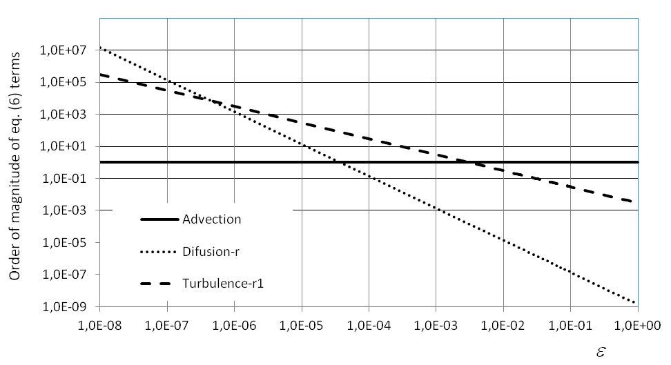 | Figure 2. Order of magnitude of the terms in eqn. (6) |
Figure 2 shows molecular diffusion effects dominating near the periphery of the plume (dotted line) and the inner distinguishing limit occurring at ε = 4.7.10-7 (at the intersection of the dotted and dashed lines). The second distinguishing limit is also evident at ε = 3.0.10-3 (at the intersection of the dashed and solid lines). The intersection of the dotted and solid lines represents the region where advection and diffusion are of the same order but where, as indicated before (Table 1), turbulence dominates. Non-dominant effects are not included in Figure 2. The problem of a pollutant plume dispersing in the atmospheric boundary layer has already been addressed by [1] Pellegrini et al. (2013), for the 3-D transient case in Cartesian coordinates. In this study the authors have successfully compared their predictions from magnitude order dominance with the analytical solution of the advection-diffusion equation with K-theory closure, obtained by [3] using GILTT (Generalized Integral Laplace Transform Technique). The authors took this analytical solution and switched off two out of three of the dominating dispersion mechanisms at a time to show where the remaining mechanism coincided with the findings from the perturbative approach. The analysis confirms the regions of dominance established by the perturbation analysis. It is noteworthy that the results of the present study are very similar to those obtained in [5]. The author’s equation for the order of magnitude of the terms reads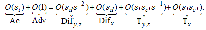 | (37) |
It can be seen that this equation corresponds to eqn. (24), if one replaces the lateral distances y and z by the radial coordinate r of the present study and the longitudinal distance x by the present study z. The distinguishing limits and the regions of dominance are identical, leading essentially to the same structure: advection dominating in the centre, lateral turbulence in the middle and lateral diffusion at the periphery. Some noteworthy differences show up in the tangential turbulence (Tθ) and second radial turbulence (Tr2) terms which are of lower order here and are obviously not present in the Cartesian coordinate system analysis. The mentioned resemblances make us confident that the present analysis is physically sound even though we do not have direct experimental data to compare with.
4. Conclusions
The present study analysed the pollutant concentration profile in plumes, resulting from the perturbative analysis of the complete advection-diffusion equation. Differently from traditional approaches that use the boundary layer and the horizontal plane as references systems, this work uses the plume itself and associated cylindrical coordinate system. The authors are aware that using the plume physical characteristics to define typical scales demand a self-consistency verification. To this end, the full solution of the plume would be of need, in order to show whether the initially used scales that were necessary to define the distinguishing limits and thus the dominating mechanisms, are consistent with properties from the solutions. Evidently it would be desirable to determine them at the present stage of work, but we postpone this task to a future work. One of the major challenges is to elaborate a method such as a recursive scheme like the Adomian decomposition [12] that would allow constructing a complete solution in analytical representation. At the present stage of development in this research, however, the existence of those scales was assumed ad hoc, simply based on known behaviour of the variables involved. Nonetheless, the analysis showed that the plume can be divided in five regions, where only certain terms of the complete governing equation dominate in first order approximation in cylindrical coordinates. This result corroborates previous conclusions of [1] with respect to the physical mechanisms dominating each region and to the ordering of those regions.
ACKNOWLEDGEMENTS
The authors wish to thank CNPq (Conselho Nacional de Desenvolvimento Científico e Tecnológico) and Linhares Geração SA (ANEEL P&D).
References
| [1] | Pellegrini, C.; Buske, D. ; Bodmann, B. ; Vilhena, M.T. . A First Order Pertubative Analysis of the Advection-Diffusion Equation for Pollutant Dispersion in the Atmospheric Boundary Layer. American Journal of Environmental Engineering, v. 3, p. 48-55, 2013. |
| [2] | Vilhena, M. T.; Buske, D. ; Degrazia, G. A. ; Quadros, R. S. . An analytical model with temporal variable eddy diffusivity applied to contaminant dispersion in the atmospheric boundary layer. Physica. A, v. 391, p. 2576-2584, 2012. |
| [3] | Buske, D. ; Vilhena, M.T.; Tirabassi, T. ; Bodmann, B. . Air Pollution Steady-State Advection-Diffusion Equation: The General Three-Dimensional Solution. Journal of Environmental Protection, v. 3, p. 1124-1134, 2012. |
| [4] | Buske, D. ; Vilhena, M. T. ; Bodmann, B. ; Tirabassi, T. . Analytical Model for Air Pollution in the Atmospheric Boundary Layer. In: Dr. Mukesh Khare. (Org.). Air Pollution. InTech, 2012, v. 1, p. 39-58. |
| [5] | Pellegrini, C. C. ; Vilhena, M. T. ; Bodmann, B. E. J. . A Theoretical Study of the Stratified Atmospheric Boundary Layer Through Perturbation Techniques. In: Constanda, C.; Harris, P. J.. (Org.). Integral Methods in Science and Engineering - Computational and Analytic Aspects. 1ed.: Springer, 2011, v. , p. 273-285. |
| [6] | Bird, R. B; Stewart, W. E; Lightfoot, E. N. Transport phenomena. 2nd edition, John Wiley and Sons, Nova York, 2003. |
| [7] | Stull, Roland B., An Introduction to Boundary Layer Meteorology. Series: Atmospheric and Oceanographic Sciences Library, Vol. 13 (1988). |
| [8] | Arya P.S., Air Pollution Meteorology and Dispersion, Oxford University Press (1998) |
| [9] | Holton, J.R., Hakim, G.J.: An Introduction to Dynamic Meteorology. Academic Press (2012). |
| [10] | Blasius, H. (1908). "Grenzschichten in Flüssigkeiten mit kleiner Reibung". Z. Math. Phys. 56: 1–37. (English translation). |
| [11] | BUSH, A. W. Perturbation Methods for Engineers and Scientists, CRC Press, USA, 320 pp. 1992. |
| [12] | Adomian. G., 1994: Solving Frontier Problems of Physics: The decomposition method. Kluwer Academic. |
 Abstract
 Reference
 Full-Text PDF
 Full-text HTML