1. Introduction

In ecology the issue of how and how much predation and competition affect the structuring of ecological communities has involved many food web ecologists in recent years.

Pressed by abrupt and unprecedented anthropogenic and environmental perturbations, there is an urgency to disentangle the ecological complexity of such peculiar natural networks [1]. Trophic chains and trophic webs have a long tradition in ecology and indeed, were addressed and drafted by authors from Sir Charles Darwin to Bruckner, Elton (food cycle) and Lindeman to mention the most popular [2,3]. Top predators, intermediate species and basal species present often constant proportions in small webs or slight scaling [4]. In general, in most predation networks abundances are inversely related to their trophic position in the food web, FW [5,6]. The species position in the network can change during ontogeny [7,8] or contexts but it seems to be rather constant at least in certain FWs with season [9]. However seasonal variability has been shown to be much greater than spatial variability in determining relative position of species in the Trophic Level, TL, stable isotopes measurements [10].

After different correlation and topological analysis of the food webs literature data, we have selected some general ecological perspectives about FWs structural complexity that could be preparatory for the management of different ecosystems in rapidly changing climatic scenarios.

Unexpectedly disparate aquatic and terrestrial communities can belong to the same connectional trend with network size whose nodes represent the number of trophic species.

Although some aquatic communities can host apex predators at higher Trophic Levels than terrestrial ones it is not clear if there are general connectional differences or hierarchies. Better understanding of how communities are shaped, considering also ancient fossil communities, has an appeal that goes beyond food webs beauty. Complex ecological communities have undoubtedly aesthetic valence but we urge to avert ephemeral mandalas and search implications for a sustainable exploitation of services and humans minimising risks of being parasitized.

• Definition of trophic network composite parameters

Typical structural food web parameters are network Size, S, and trophic Links, L, and many composite parameters have been proposed by FW ecologists [11-14]. In this analysis, we present empirical correlations between a basic modified parameter of communities, linkage density bottomless, LD_bl, or reconnecting with our previous analysis [15]:

in which all links are spread between consumers, and topological connectance defined as:

i.e. the maximum number of potential links of the web for consumer species. This parameter is considered more suitable for comparing topological links from aquatic and terrestrial habitats with slightly comparable but different number of resources (trophic aggregation).

Producers or number of basal species, B, are those species that start the flux of energy with no incoming links. Top predators’ species, Top or T, having no outgoing links, are only by definition not predated by other species, while intermediate species, Int, display both ingoing and outgoing links [6]. Interestingly in trophic chains connectance or connectedness, defined as:

is identical to:

namely, the bottomless connectedness for the FWs with the same S. Mainly bottomless parameters were chosen in the present analysis considering that they could be of greater value while focusing on link distribution among higher Trophic Levels species. In order to quantify a flexible attribute of ecological organization of real communities, we focused on the predator-prey interactions while neglecting sometimes ‘dead-ends’ trophic species which are not directly sustaining predators at the highest Trophic Levels; some basal species nodes could represent parts of primary producers and become a misleading indicator by inflating the consumers network size and lessening C'.

Following an analogous definition [15], although utilizing a parameter of greater variance than L∙S^-2, its average value for certain communities attested close to 0.5 that could be of theoretical significance as a threshold or bound.

Plotting didactically m_bl vs m_bl*, allows to quickly capture concomitantly constant un-weighted connectance (i.e., slopes of the lines, excluding cannibalistic loop in Figure 1) and constant linkage density (green dashed line) sampled ecological communities in small intervals.

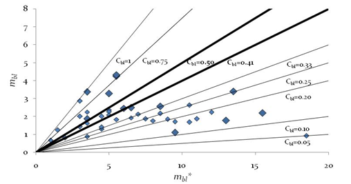Figure 1. Effective link density vs topological normalized connections. Data for the communities from constant environments are represented by bigger diamonds. All communities belonging to the approximate interval, 0.05 < Cbl < 0.96 can be graphically represented by the family of lines passing through the origin. Hypothetical mean (Cbl = 0.5) and median (Cbl = 0.41) Cbl lines and values have been bolded. Average connectedness Cbl = 0.40 (number of communities = 40), for bottomless communities (excluding basal species), was slightly higher compared to the C’ = 0.30 value for the same 40 communities that was identical to C’ for the whole sample of collected FWs (n = 113). Interpretation of the constant Link Density communities (dashed green line) was tentatively re-examined in alternative to FWs pictorial constraints. Raw data reported in [16], collected in [17,18]

We suggest to avoid connectivity denomination for either C’ or C_bl in particular when they are not explicitly defined, since this term after 1984 has become even more fundamental in landscape ecology [19,20]. We opted for another connectional parameter that at least in ideal food chains does not vary increasing the number of trophic levels (bottomless link density: ) and is at least unitary with short-circuit or food web-like structure.

Interestingly the significant trend of increasing m_bl with N - number of trophic levels or height - or maximum chain length, MCL, was not apparent when plotting Average max number of Chain Length, ACL, (n =40 homogeneous community selected by [16]) although r = 0.781 and in a revised sample [5] the correlation of these two food web lengths was even higher with r = 0.938 (n =98, one-tailed p<<0.001, d.f. = n-2).

Indeed, communities of different sizes can be characterized by equal C_bl values (Table 1, Appendix A).

1.1. Simplifying the Ecological Complexity

Ecological analogies with digital librarianship warn us about writing a manuscript without a proper software or permanent cross reference tool that automatically update number and position of references. If anthropization inflicts drastic changes at every scale, from local to planetary, it is unlike that we could tell how ecosystems will react or if community will persist or reassemble when biotic interactions (disordered or mismatched references) will be lost or greatly rearranged without understanding the basic semantic of simple topological networks.

• Species aggregation, body size trait/predator prey ratios to predict community trophic levels

Un-lumping basal trophic levels in FWs do not increase the average number of TLs but this procedure can clearly diminish them [21]. If the communities have constrained topological links, then we expect a strong sensitivity of MCL to m_bl. Indeed, the empirical observation that most communities have short chains, their “extreme length limit” does not imply an energetic limitation allowing to reach the top of the chain (see [22] and references therein).

In spite it was shown that increasing the number of TLs will delay the recovery time from perturbation (resilience) of the FW [23] and dynamical instability is reasonably dependent on trophic architecture. However, efforts to make ‘atomistic’ dynamic models less phenomenological must be acknowledged (wider list of hypotheses in [12,24,25]).

Recently McGarvey et al. [26] with trophic energetic efficiency considerations and by extending allometric scaling of production rate versus body size, could explain why pelagic ecosystems could sustain the 5^th trophic level with a minimally rescaled sample of those communities [27]. The proposal of body size-food web structure integration is not new in food web literature [28,29] but it is original how the more robust empirical FW components and groups are assembled and how body size affects the variability and persistence of food webs [30-33]. In dealing with interaction strength and stability in a real food web, predator-prey body mass ratios have been proposed as a surrogate-correlate of the interaction strength (e.g., [32]). This approach, considering the occasional occurrence of complex ‘anomalous’ (not allometric) trends, needs careful examination.

Information being scarce and rather variable about species abundances (trivariate analysis in Ings et al. [34]) or energy fluxes between TLs, most of the literature concentrated on theoretical modelling in search for robust approximations or static analysis of ‘first-generation’ food webs [35,36]. In this context, linkage density, as a partial indicator of food web complexity (S∙C), has been demonstrated by N.D. Martinez using the Kendall’s nonparametric tests, to increase with S in communities where the number of species, S > 54, and widely thought not to be scale invariant [4]. Significant trend of normalised number of nonzero links, L/S, and %B has been also observed in [5,37] but L/S was shown to be larger in food webs with large S because of the uneven aggregation between the communities (see also the sampling effort bias in [38]).

Surprisingly, recent analysis found that the functional properties of FWs were preserved over a large portion of the aggregation gradient [39]. Definitely not only body-size could interpret MCL as parsimoniously proposed [37].

1.2. Topological Structure of Ecological Networks: Communities from Stable vs Variable Environments

Topological indications of ecosystem persistence or health could be derived from the calculation of fine-scale structural parameters in comparable contexts with only one main or few environmental or relational variables perturbations or most diversified cross-habitat comparisons in either ‘constant’ or ‘variable’ environments or gradients [34]. Pioneering papers by J.E. Cohen [29] and F. Briand [17] evidenced the significant difference of Connectance, C, between communities from stable environments and those from fluctuating ones. It was defined as:

where n replaces S (number of nodes or Species) for a more intuitive denomination that does not generally interfere with statistical symbols as does n with sample size. As F. Briand theorised, the greater connectedness in communities from constant environments might be even associated with high interaction strength, violating the condition for dynamical stability [40]; being the probability of environmental disruption low, this behavior appears acceptable.

Schriever [41] by means of a multivariate approach analyzed effects of the environmental variability on ponds concluding that MCL responded to both multiple environmental variables (e.g., hydroperiod, T) and species assemblage. Therefore, interpretation of food webs structure should sometimes not disregard the historical contingency.

Remarkably MCL significantly correlated with S in none but short marine estuarine group (r = 0.815, two tailed p = 0.001, n = 12) [5] reinforcing the fact that the overall LD-MCL correlation is not obvious. In a sample of insect dominated communities, (see par. 1.3, Hypothesis of a trophic level threshold for trophic pathways), when considering only independent observations, even the modal chain length, lost statistical significance in the log-log correlation with S (Bengtsson J., personal communication).

Here we expand the ecological implications of the empirical correlation analysis between LD and MCL delimiting LD intervals of validity (see list of parameters in Appendix A).

1.3. Topological Structure of Ecological Networks: Aquatic vs Terrestrial Communities

Higher degree of trophic specialization in large terrestrial communities should allow more Trophic Levels in a food chain from a simple energetic calculation assuming constant ecological efficiencies and an estimated five times greater photosynthetic production [see [26]]. Theoretically more biomass would be available for sustaining further Trophic Levels with their emergent ecological patterns from less sideways routes. Despite higher average feeding specialization (i.e. lower connectance) in terrestrial communities than in aquatic ones, diet breadth variation was recognized to be dependent not only on species richness and habitat type but also on the variability in the resources and sampling effort (see analysis of insect herbivores in [42]).

Only in lakes a latitudinal gradient of the scaling of LD, generality (gen) and vulnerability (vuln) with S was evidenced [43]).

The terrestrial food webs are typically considered shorter because of different organism size and dynamics of the bottom resource and primary producers (phytoplankton vs plants) and an inferior ecological efficiency at the base of the trophic pyramid [15], [44].

Interestingly we were expecting to find communities differences more easily identifiable from charismatic species studied in greater detail while herbivorous richness and intensity are becoming central for answering many ecological issues [e.g. [45], see reference 46 therein].

• ‘Size Ambivalent’ Communities (SAC)

Apart from the Malaysian Rainforest and Canadian Willow Forest, terrestrial communities, from the Briand collection [17], were large according to our group size classification (S ≥ 15). These two small communities (low S) of first-generation food webs are characterized by the same logarithmic trend of realized links vs maximum potential links of large communities but belonging to the small size group (S < 15). Their structural link density scale as if they were somehow large or ‘size-ambivalent’. A similar trend has been exhibited by the aquatic Pamlico River and the Marshall Reefs. Such communities belong to the same global pattern of increasing MCL with m_bl as anticipated in our abovementioned paper [15], till a critical linkage density (m_bl) of around 2.5 close to the most common region for the 40 communities (see par. 1.3, Hypothesis of a trophic level threshold for trophic pathways and par 3.1, Herbivores diversity and proportion as a proxy for TLs). We have introduced SAC notwithstanding the dubious uniformity of aggregation of the trophic species/functional groups of this collection of food webs since after redrawing these food webs interesting values of C_bl ~ 0.4 were obtained (see Figure 1).

For this subgroup of communities “extreme trophic levels” were derived without the need to know all links but only a fraction of species, namely it holds:

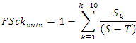
where Number of herbivore species /S.

In SAC Log LD_bl = 0.3 the sample link density mode, typical of species rich communities could indicate, under certain assumptions, a constraint rather than a trivial artifact (see averaging procedure in par. 3.1, Herbivores diversity and proportion as a proxy for TLs).

• Functional diversity, trophic interactions in modern or ancient webs

Attempting to address the elucidation of the profound macroscopic differences between aquatic and terrestrial communities in less habitat specific terms than T.W. Schoener [5] did, we presented different pattern of trophic levels correlation with LD between aquatic and terrestrial community webs not mentioning ‘obvious’ hypothetical causes like water limitation or more TLs in the latter communities being functionally rich or peculiar [15]; furthermore adaptation to land and environmentally huge differences (e.g., ecological efficiency, oxygen availability, and basal groups peculiarities) were expected to be somehow reflected also in the community structure and predator-prey flexible interactions.

Interestingly analysis of fossil ancient food webs from the 48 Myr-old Messel deposit found a 5% of specialists in Messel Lake while 14% of taxa feeding on one taxon was reported for Messel Forest with almost all parameters of the trophic structure of the Messel Lake web that fit within the ranges observed for extant webs [45]. Investigations of the topological structure of terrestrial and aquatic communities (see [44,46]), by comparative analysis, are making scientists foresee some theoretical-empirical rules of their functioning, from pattern to processes (e.g., see detritus-based subwebs by Rossi et al. [47]).

Schalk et al. [48] studying tropical pond communities concluded that unrestricted diets and plasticity enables consumers to exploit a broad range of resources and promote species coexistence suggesting that high diversity in tropical ponds does not necessarily translate into specialization of trophic function.

Traditionally whenever two or more species are preyed upon by exactly the same set of predators, and prey upon exactly the same set of prey, in each food web, tropically identical species were lumped together as one [49]. This analysis showing the singularities of different groups of freshwater ecosystems focused on lentic and lotic communities from different biomes but of comparable network size (8 < S < 23). Commenting on how a brief appearance of an opportunistic top predator could reshape the community structure, top down cascades were observed in aquatic ecosystems [50,51] but also in terrestrial ones [52,53].

Mathematical modelling that incorporates both top-down and bottom-up cascades are promising tools to interpret different propagating effects in FWs [54,55] and especially widespread anthropogenic impacts at all TLs [56].

• Hypothesis of a trophic level threshold for trophic pathways

The isometric trend for lakes and environmentally hyper-variable communities, after calculation of bottomless parameters, could suggest the presence of some sort of compartmentalization to counteract the higher risks of predation expected as indicated by their high relative link density. An opposite hypothesis conceives many lake’s vulnerable species saved from extinctions as a consequence of the weakening of the intensity of such predatory links due to the high number of alternative preys. On average there could be a tendency of reduced risk of species extinction when the number of trophic pathways is greater. However, we have drawn indication of a limit to the number of trophic pathways with TLs from a collection of insect food webs [57] after excluding gall FWs with parasites; without such exclusion a perfect linearity of trophic pathways vs TLs was observed (R² = 0.99). To complicate the interpretation, link relevance in terms of energy flows does not necessarily parallel strong interactions sensu R.T. Paine [58].

Figure 2 summarizes different trends of link density where m_bl can either increase or decrease with network size.

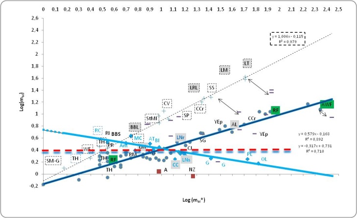Figure 2. Across habitats invariance and scaling of connectedness. Bottomless link density (mbl or LDbl) vs topological connectance (mbl*, LDbl*) for the 40 communities (in red Arctic sea and salt meadows New Zealand communities) collected in [17] and [18]. Labeled in dark blue trend for communities from ‘variable environment’ (ii) and in light blue opposite trend for most communities (bold) from constant environment (iii). CC: Crocodile Creek, LNs: Lake Nyasa sandy, LNr: Lake Nyasa rock. Another collection of recalculated comprehensive food webs bottomless parameters were added [57]. AT: Arctic tundra, PL, OL: Pine and Oak logs, TH: Tree Holes, G: Grassland, LRL: Little Rock Lake and other large lakes’ food webs in grey (AL: Ancient Messel Lake fossil community, Rain Forest and Ancient Messel Forest (AMF) in green (data of comprehensive food webs from [1]; ancient food webs from [45]). With Plus indicator all isometric Cbl food webs, mainly lakes and creeks (i). Minus indicator for linkage density of ‘comprehensive food webs’ (e,g. Ythan Estuary with parasites, YE). Dark blue dots for variable communities with refuges (rainforest, ancient lake - not corrected), LNr, Reef Marshal,RM and Sea Grass, SG. In red a dashed line threshold for mbl around 2.5 links / trophic species

A pattern of constant connectance was deduced by calculating this parameter for certain cumulative ‘comprehensive food webs’, namely it holds:

(i) C_bl=10^-0,115 =0.77~ ¾

(environmentally hyper-variable communities - dashed line)

(ii) C_bl=10 ^{-(0.42logLD*+0.163)}

(heterogeneous environmentally variable communities - LNr- dark blue)

(iii) C_bl= 10 ^{-(1.339logLD*-0.748)}

(open-space environmentally constant communities - CC, LNs- light blue)

Our choice, to focus only on few parameters of predator-prey interactions, without considering parasitic and collaborative networks, derived that none of us, neither our small group of authors, could dream of winning such a triathlon competition. The huge effort in addressing such a broad research area and the conflicting effects on performance of trying to improve in more than one field all at once, parallel different group of muscles trained during swimming, cycling, running, that cannot excel in all three sportive disciplines.

• Functional diversity in different habitats

Species richness follows an inverse biogeographic trend with latitude and its correlation with habitat heterogeneity and environmental gradient of energy were reported for mammalian, fish and bird species though more robust analysis are underway [59]-[61].

Trophic species rich communities are more frequent in the dark blue trend (see Figure 2) of heterogeneous variable habitat (ii) whereas ‘open-space communities’ are found mostly in the light blue trend (iii). Clearly pattern differences are not only in relation to observing large or small networks but conservation or management decisions could benefit from network analysis starting from basic parameters and simplest FWs snapshots (see [6]).

2. Perspective from an Innovative Methodology

Max chain length occurs at the crossroad of energetic and connectional parameters. Conceptual basis for bridging energetic and connectional aspects of food webs combining reductionist premises and parameters to holistic observed complex ecological networks were provided [15]. Recently it was stated that complex ecosystem networks consist of a multitude of weak connections dominated by a relatively few strong flows and trophic depth (a measure of number of TLs) was formalized and presented, under certain assumptions on the degree of organization of the ecosystem, in a linear correlation with trophic breadth [62]. Here, in a functional topological framework, a new set of parameters were defined by us to address analytically the issue of linkage density and levels complexity of trophic webs. FSkc_y, the complement of the relative cumulative fraction of species (in + out) normalized by the total number of vuln and gen links, points to testing species and trophic transactions (sensu [63]) interplay.

Without measuring directly energetic fluxes of environmental networks, we could extrapolate both connectional and indirect energetically related parameters, oriented by an analogous contextual alternating role of forms and contents in social sciences. This procedure allowed us to progress further towards the integration of energetic and connectional aspects of food webs and to circumscribe hypothesis discriminating macro-descriptors of exemplary lacustrine food webs from the same location, the African Malawi-Nyasa-Niassa lake [64].

The functions FSck_vuln and FSck_gen were defined as:

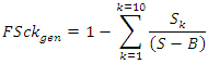where to each k (number of link-in or vulnerability link) corresponds a certain number of nodes or species in the S×S matrix that are counted and summed up from LD₁ till LD₁₀ where all predatory links are exhausted. Top predators were not subtracted from the denominator assuming that also top predators are somehow vulnerable and they were not counted in LD₀ associating always 1 to FSck initial condition. The function FSck_y was calculated according to the following form:

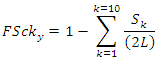where in this case to each k corresponds a certain number of nodes or species that are ‘interwoven’ by a certain number of total ingoing and outgoing links (see Figure 3).

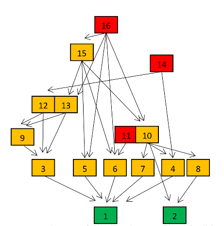Figure 3. Lake George FW. Nodes are trophic species, links represent predator-prey relationship. Green nodes indicate plants or single cell producers. Intermediate Species and Top Predators are reported in orange and red color, respectively

3. Results

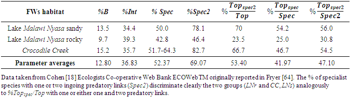
In Figure 4 structural parameters, the cumulative fraction of species presenting average community vulnerability at each k number of predators (green thick trend), are plotted in relation to another newly defined parameter (yellow thick trend) whose complement of cumulative fraction of species intercept at MCL+1. We propose a critical LD for LNs at 3 instead of 4 (Figure 4). In CC and LNs habitats belonging to the opposite pattern of connectance and species richness of Figure 2 with respect to LNr, MCL could be more precisely associated with a minimum of predatory pressure (highest filled red dots) and an inversion of the blue, yellow LDs thresholds. It is important to note that Int average ‘vuln’ is also much greater in LNr than in LNs and CC and C_bl value of LNr is about two times greater (see Table 1, Appendix A) although all these communities were sampled in the same location. We hypothesise a minimization of predatory pressure for all communities not only from compartmented habitats and energetic constraints categorisation of extrapolated LD_y-y < LD_v-y for LNs and CC or LD_y-y > LD_v-y in the case of LNr (Figure 4). Computed structural parameters are reported for the three communities investigated in greater detail from the Lake Nyasa-Malawi-Niassa (known in Tanzania-Malawi-Mozambique respectively), the southernmost lake of the Eastern Africa Rift system (Table 1, Appendix A). More typical parameters of food web literature, %T, %B and %Int are associated with LD_y-y and only % Int is concordant (Table 2, Appendix A).

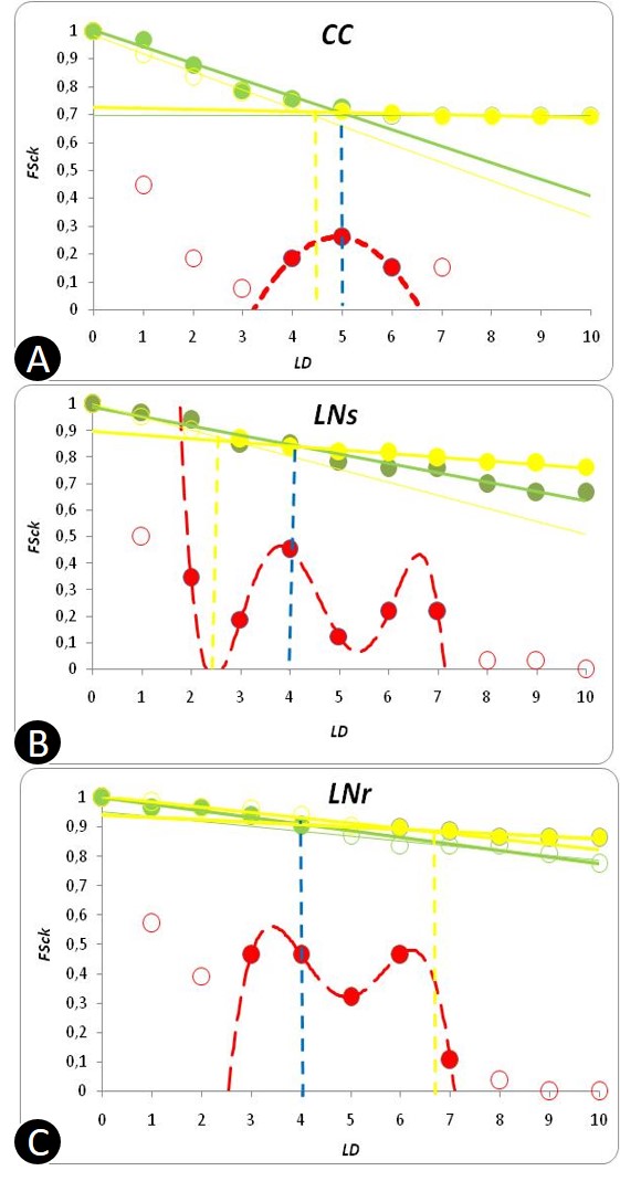Figure 4. Structural and surrogate energetic parameters of exemplary food webs

To summarize some definitions, we have drawn an anonymous food web with S = 16 and L = 25, TLs =MCL = 5 (depending on the different first level attribution). C = 2 ∙ 25 / (16∙15), C_bl = 2 ∙ 25 / (14∙13), LD = m = number of links / 16 and LD_bl = m_bl = 25 / 14.

Simplified schematic food web / ecological Network

1. Basal species (only vuln links)

2. Basal species (only vuln links)

3. Intermediate species (vuln and gen links)

4. Intermediate species (vuln and gen links)

5. Intermediate species (vuln and gen links)

6. Intermediate species (vuln and gen links)

7. Intermediate species (vuln and gen links)

8. Intermediate species (vuln and gen links)

9. Intermediate species (vuln and gen links)

10. Intermediate species (vuln and gen links)

11. Top predator (only gen links)

12. Intermediate species (vuln and gen links)

13. Intermediate species (vuln and gen links)

14. Top predator (only gen links)

15. Intermediate species (vuln and gen links)

16. Top predator (only gen links)

§ Predator-prey adjacency square matrices, allows to draw the FW starting from A_ij elements (1 trophic relationship: 0 no link between the trophic species)

§ Calculate composite network parameters and fractions

§ Apply our new method described in par. 2 to species rich communities

§ Links are not weighed but trophic position can be calculated (simplified FW from [65])

A newly defined parameter FSck_y (yellow dots), complement of the Fraction of Species k-connected (in+out) normalized for the total number of effective matrix gen and vuln links is plotted (par. 2). By fitting initial values (low LDs hollow yellow dots) of this newly defined FSck_y and final values (high LDs filled yellow dots), LD_y-y is obtained by extrapolating a LD value from the two linear fitting equations. The intercept of the FScK_v-y and FSck_y-y trend lines individuate different linkage density thresholds. The Maximum Chain Length values are in relation to LD_v-y ̶ 1. This parameter corresponding to the abscissa value where the trend of the complement of the cumulative fraction of vulnerable species (FSck_v low LDs, green filled dots) intersects the trend of the complement of the cumulative fraction of the species with link-in plus link-out normalised by total number of links (pred+vuln) FSck_y (high LDs, filled yellow dots). Interestingly to this value corresponds a minimum of predatory pressure for arbitrarily simulated (shadowed red dots) FSck_g according to absence of vulnerable species (or a single species) at that LD_vuln. Hollowed red dots were those FSck predatory values not included in the trend. Lake Nyasa-Malawi-Nyassa food web swampy CC (A), sandy LNs (B) and rocky LNr habitat (C). Data from Cohen [18] taken from Fryer [64].

3.1. Connectance, Linkage Density and Height of Ecological Networks

Searching for connectional thresholds, we fitted community’s Height (MCL) vs LD_bl with a nonlinear polynomial model of the 4^th order by interpolating average linkage density values for each TL (Figure 5). Highest MCL values are of extreme environment communities, with different network sizes, and possibly more subjected to climate warming threat.

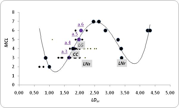Figure 5. Maximum chain length vs link density. Maximum number of trophic levels, MCL, as a function of LDbl (n=16 communities). To draw the fitting curve, data approaching to LDbl equal two, where averaged for each trophic level a.3, a.4, a.5 and a.6. Mostly terrestrial communities with LDbl closer to the abscissa of MCLmax were excluded from LDbl average calculation corresponding to MCL=4 (also Lake Abaya [5] was not considered). Only exemplary lacustrine FWs (LNr, LNs, CCand LG) were indicated in grey in the graph. Communities not averaged (smallest dots). MCL of Ross Sea was taken from [26]. Large size black dots for communities that were included in the polynomial fitting (data from [27])

• Herbivores diversity and proportion as a proxy for TLs (obvious for chains)

Arctic and Antarctic communities display also large number of average trophic levels (ACL) and a significantly reduced %H (the ratio of herbivorous and detritivorous species to other consumers). Consumption by Herbivores in terrestrial ecosystems was shown to be on average three times smaller than in aquatic ecosystems for a given level of primary productivity [66] and size-consumption scaling of herbivores could indirectly explain MCL in our lake case study. In fact, management of terrestrial ecosystems is starting to tackle both herbivores diversity and secondary productivity in different ecosystems [56]. Furthermore J. Lubchenco & B.A. Menge [67] attributed to herbivores a potential controlling role of intertidal community succession.

With selected literature data at hand [27] we refer to broad categorization of herbivores in a unifying perspective for community’s “extreme trophic levels” approximation. We would expect a faster decrease in ACL with in terrestrial than in aquatic communities. Future refined studies, analogously for predators, could consider mobility of the species, contrasting browsers versus grazers, ectotherm versus endotherm herbivores and integrating different species traits into ecological networks.

• Stratigraphy in food webs (trophic levels)

According to the results of Figure 4 we defined a new synthetic species density Y_N-1 parameter computed as the number of species at the level N ̶ 1 divided by the Potential contiguous Weighted inter-level interactions, PcWii (Table 3, Appendix B). The greater variability of this partial ‘vertical’ community parameter should probably be intended as a measure of independence from and adaptability to the environment and not of instability of the communities with greater height (number of TLs). Furthermore, energy-limited communities belong to the main axis of an ellipse where increasing C_bl could lead to a constant increase of the Y_N-1 parameter. S_N-1 / (PcWii) is plausibly minimized for all three species rich communities of Lake Nyasa-Malawi-Niassa and maximized for mostly terrestrial communities at C_bl ~ 0.2 (values in Table 1, Appendix A). In this regard it was shown that an increase of percent omnivory, consequent to habitat coupling in relative smaller lakes, brings about a shortening of food chain length after increasing the accessibility of preys lower in the food web [25]. A food web could shrink in terms of species reducing its ACL but increasing connectance and hence lengthening their chains in favorable conditions like those occurring during seasonal or inter-annual favorable conditions [see [68]]. Other considerations about habitat type, stability and complexity were discussed by Shurin et al. [44].

4. Discussion & Conclusions

Comparative analysis and modelling of Ecological Networks offer a new perspective for a better understanding of communities as a whole. Rational management of natural reserve areas [69-70] and more in general unravelling the complexity of real ecological communities could be addressed with different network approaches possibly having matured awareness of potential pitfalls [1,34,62].

Efforts to make coherent the trophic level concept are encouraging and constructive [35,51]. Often its heuristic power becomes evident only above a threshold where certain structural parameters cannot be much relaxed otherwise S.H. Cousin’s considerations cannot go unheeded [7]. Whenever possible existing food webs should be updated, and homogeneity of data more than exhaustiveness of resolution pursued to meet more functional than compile project’s aim.

Gaining insight on the relationship between trophic web structural parameters and indexes of stability, persistence or services/health (indirect measure is easily obtained from catches estimated by fisheries) of an ecosystem should complement traditional ecological studies in responsible decisions of re-wilding and re-wiring.

Therefore, a list of key points re-analyzed follows:

§ Architecture and patterns of ecological networks are meaningful for the interpretation of many different general ecological outcomes of trophic species number (coexistence) and connectance that could help explaining the reported constant [13,70-72], power law C findings [12,13,40] and also opposite link density (LD or m) pattern in diverse aquatic and terrestrial habitats [68,73].

§ All-seasons communities belonging to the ‘hyper-variable’ trend, free to increase their S, optimize their connectional network (C ~ 0,75) reflecting opportunistic foraging if not methodological biases. Species normally attract and interact with other species and adding ‘guardians’ to ‘rebel species’ could avert monopolization of the habitat (e.g., Pisaster starfish-effect on a strong competitor for space, Mytilus [58]). According to Martinez [13] larger communities do not display smaller C values after normalization is carried out (see also Figure 2).

§ A fossil paleo-community structure, Messel Shale, featuring lake and forest food webs, belonged to the same trend of link density vs topological links of extant communities from variable environments with lake having ~ 3 times more strictly specialist fossil taxa [45]. It could be interesting to extend this analysis by Dunne et al. with different indicators of specialization (see different ranking in our case study Table 2).

§ After recognizing the presence of at least two different linear patterns of link density with food web size, log-log scale, we focused our analysis on species and link distribution of three exemplary lentic communities from the same location (LNr and LNs, CC). A new adjustable tool (Figure 4) was used to integrate trends of link distribution with effective network size and complexity (see degree distribution in [1,34,74]).

Manipulative experiments have shown that the introduction of a generalist predator will often weaken other competition-based coexistence mechanisms resulting, whether by habitat segregation or indirect interspecific interactions, in competitive exclusion [75]. Satiation of the predator or switching may be more relevant for the dark blue pattern (Figure 2), where piscivorous fishes especially those that consume prey whole and provide extended parental care regularly experience long periods of empty stomachs [76].

§ ‘Comprehensive FW’ increasing the reliability of patterns led us to estimate relative ‘missing links’ between mainly terrestrial communities and mainly lacustrine ones (data file kindly provided by Prof. J. Dunne); our attempt to convert communities from different trends resulted in an increase in the LD parameter of ~ 5 times (i.e. range from 2.6 to 10.3) or a corresponding reduction in topological links of around 20 - 40 links/species after antilog transformation of the log L - log L* data trend (references in Appendix C; see also [77]).

§ The simulation of low exerted predation pressure at low k-species vulnerability to support the localisation of maximum effective TLs where ‘predatory pressure’ is reasonably reduced for all communities suggests a more relevant bottom-up TL control in the sandy zone or creek than in the rocky zone of this great African lake (Figure 2; FWs in [64]); burrowing could help prey hiding only from visual predators some of which ambush, whilst rocky barricades with their numerous refuges could allow a more efficient and reliable top-down control (Figure 4).

§ ‘Predatory pressure’ should be intended not as interaction strength or intensity but simply indicative of a niche or network condition where few consumers (Top or Int) realising predatory links of degree k pander vulnerability.

Most species, when not masking, interact in a food web by attractive and deterrent signals.

Defenses of plants are much more common on land environment [78] and indeed feedbacks are widespread at different levels of biological organization [79,88].

4.1. Examples of Camouflage in FWs

As an unusual example of anti-predatory tactic, animal changes in brightness could reduce detection probability of crabs [80,88] and notwithstanding ubiquity of mimetism (e.g., Figure 6) the adaptive significance of carapace geometric patterns is still under field and laboratory experimentation.

Different camouflage strategies minimize signal to noise ratio [81], both background sand matching in estuarine cryptic juveniles and possibly displaying disruptive markings in Carcinus aestuarii juveniles frequenting structurally more heterogeneous habitats have been observed in the western side of the North Adriatic Sea (45° N, 12° E) (Valandro L.R., in preparation). Quantification of effectiveness of resultant avoiding predation by field experiments or going further the commonness of camouflage in both aquatic and terrestrial habitat, and different contexts, could quite soon open up innovative research avenues with integrative methodologies at the moment only prudentially listed in food web modelling [26]. All species are likely vulnerable at some stage including apex predators.

Furthermore, cannibalism and damages by bigger conspecifics should necessarily be included in network modelling functional responses, returning species identity relevance, here only indirectly manifested.

All species are vulnerable and mimetism is ubiquitous but never obvious. In Figure 6, panel A a cryptic Carcinus juvenile with three white triangles and a black spot in the dorsal side of the carapace remains motionless but only partially under the sand. If conspicuous to visual predators such white triangles or dark spots when not corresponding to any search image of their natural predators could be interpreted as a ‘cognitive mimetism’ allowing the crab to avoid recognition by visual predators or harassers. A spotted newborn lamb (Figure 6, panel B) and a copepod (Figure 6, panel C) are common species of terrestrial and freshwater habitats.

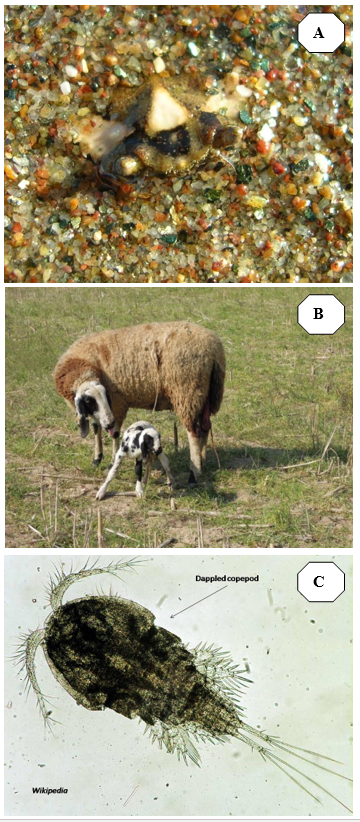Figure 6. C. aestuarii juveniles (estuarine-marine), newborn lamb (terrestrial) and a Cyclopoid copepod (freshwater) on panel A, B and C, respectively - 6C adapted from https://it.m.wikipedia.org/wiki/Cyclops US Environmental Protection Agency

Consumers interact less effectively with camouflaged species especially during development, whereas community predation pander vulnerability mainly in crowded habitats. Camouflage is a ubiquitous mode to avoid predation and we would expect to behold its optimal modulation at different trophic levels in different contexts.

4.2. Anti-Predatory Perspective and Fraction of Primary Consumers

Notwithstanding our awareness of possible consistent subsidies among habitats, aquatic and terrestrial communities have been compared from an anti-predator perspective and empirical data [66] were confirmed with food web parameters different trends .

Whenever herbivory seems to play a role of a determinant parameter in structuring food web complexity, herbivores and animals mobility trait could be crucial to reveal the mechanisms.

The upland moa, an extinct though quite generalist herbivore of New Zealand, was probably migrating seasonally thus becoming the “highlander” of the flightless moas; it had probably a speckled appearance (not unique to Megalapteryx didinus) and it could be interesting to prosecute the reconstruction of terrestrial ecological networks of moas from coprolites, gizzard contents, isotope analysis to contrast what we envision was the more wide, complex and persistent heterogeneous habitat according to the framework here proposed or see inverse primary consumer size-ACL hypothesis [82]. Size of large and mega herbivores is often also anti-predatory but it seems reasonable that avoiding human hunting was pivotal more than avoiding predation by Haast eagle or protecting eggs considering that, although exceptionally coloured, eggs of M. Didinus were the smaller and thinner among the moa species [82].

Longer lower limbs in hominid populations could allow to reach easily and more economically terrestrial and aquatic feeding sites. However, approximate average specific power calculations were provided considering arm movement biomechanics and length to be a driver for human evolution in hunters and fishermen [84] and postponing prey target size or sportive launching accuracy to future analysis.

Whether networks of mutualists are possibly more often impacting communities on longer temporal scales, we expect active involvement of abundant parasites and virioplankton in particular to exert their multiple effects in shorter timescales [85].

4.3. Trophic Levels Extreme from Cumulative Distributions of Links

The analysis of link distribution and the definition of two parameters with energetic and vulnerability connotation (FSck_y, FSck_vuln) provide a new interpretation for maximum chain length of food webs (Table 1, Appendix A). Energy trends in combination with vulnerability patterns seem to individuate the “trophic level extreme” of a food web that is already implicit in the matrix information; in this approach overall distribution of links enriches the framework and could add directional predictive power by changing the fraction of species involved after different perturbations or somehow changed ecological contexts. Community Height (MCL) is possibly not energetically constrained in LNr where aufwuchs (algae plus microfauna) is omnipresent [64]. Analogously to other food webs of the dark blue trend of Figure 2, although environmentally variable, they could have continuous high-quality food supply. The observed greater MCL for CC could be in relation to the reduction in Top specialisation as compared with LNs (see Table 2, Appendix A and Figure 4) by a reduced vulnerability of the further stratified community [see [36]] the extra carnivorous cyclopoid copepods node. Other herbivorous cyclopoid species are abundant in Lake Nyasa sandy and rocky shores but Macrocyclops was exclusive of Crocodile creek ecological region [64]. Interestingly a shorter modal chain in CC was reported [57] giving credit to Briand & Cohen food web structure simplification and supporting the Eltonian general observation of low number of TLs especially at warmer tropical latitudes. However a deeper analysis is needed to explain the low C value of Crocodile Creek community and the text paper from which the food webs were originally taken [64] reporting generalist species in the weedy lentic CC in order to survive shortage of food during flooding events of the rainy season.

The number of TLs increases with link density between intervals at least in this small sample (Figure 5). We expect highest Height of whole ecological communities as already presented for zooplanktonic lacustrine food webs at low zooplankton Species Packing (range of SP in Table 3, Appendix B). A concomitant large network size and high ACL is theoretically allowed for LD^-1 close to 1 (trophic chain-like efficient energy transfers) and LD ^-1 ~ C_cr (data not shown) analysing data from lake Okeechobee, part of a vast protected aquatic ecosystem including the Florida Everglades [68].

To our knowledge not many conclusive results have been obtained by the exploration of ecological networks assembling process [41]; however, data are growing from frequent cases of species extinctions or threatening invasions.

It would be interesting to investigate the temperature effect on disparate lentic ecological networks and macro-descriptors. Hierarchical communication among sub-webs and the whole food web in lentic systems from the same location could also be a topic to investigate with long temporal series datasets from experimental surveys and satellites. Probabilistic (trait matching) and Bayesian approaches have been recently addressed in the ecological network discipline. Further work, assisted by new algorithmic techniques and programs and including in models organism traits [86-87] will tell us how much mathematical ecologists are bringing us closer to bio-signalling and biocenosis’ understanding and safeguard.

ACKNOWLEDGEMENTS

We would like to acknowledge Prof. JH Cohen for authorizing us to utilize matrix data of communities from Ecologists Co-operative Web Bank (ECOweb TM) and Prof. J Dunne for providing taxonomical information of the comprehensive FWs. Prof. A Minelli improved the structure of the manuscript and provided crucial bibliographic information and discussions about complexity of organisms at different levels of organization. Prof. L Colombo, Prof. J Reynolds and Prof. TW Schoener commented the manuscript with clarifying feedbacks. We are indebted to Prof. B Patten for improving a preliminary version of this work. Many thanks also to Dr. William Irwin for his suggestions.

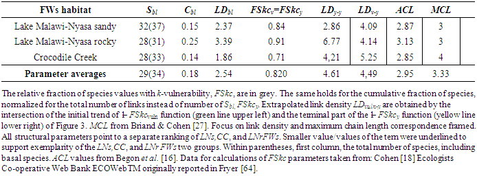
Appendix A

Parameters of exemplary regions of Lake Nyasa-Malawi-Niassa

Table 1. Food webs bottomless parameters of different lentic habitats from the same location (Malawi-Nyasa-Niassa)

Food Webs structural parameters of three Lake Nyasa habitats

Food web number 33, 38, 39 of the Briand and Cohen collection - Smaller value/values of the tern were underlined to support exemplarity of the LNs, CC and LNr FWs two groups. The differences between %Top species are very small while %Top_bl are inverted after the exclusion of the resources from total number of trophic species. %Top is higher in the rocky ecological region of the Great African lake (54.8%) and smaller in the sandy and crocodile swampy areas respectively (54.1 and 54.5). Average %Top is 54.47 (n=3). %Top_bl were 60.7, 62.5, and 64.3 (Average = 62.50%; n=3).

Table 2. Food Webs structural parameters of different lentic habitats from the same location (12° S, 34° E)

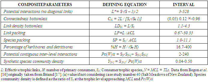
Appendix B

Further structural parameters definition and intervals

Table 3. Further structural parameters definition and intervals

Appendix C

Authors and acronym of ‘comprehensive trophic networks’

Coachella Valley, CV (Polis 1991), St. Martin Island, StMI (Goldwasser & Roughgarden 1993), G, UK Grassland (Memmott et al. 2000), SP, Skipwith Pond (Warren 1989), Bridge Brook Lake, BBL (Havens 1992), Little Rock Lake, LRL (Martinez 1991), Canton Creek,CCr, and Stony Stream, SS (Townsend et al. 1998), Chesapeake Bay, CB (Baird & Ulanowicz 1989), St. Mark’s Estuary, StME (Christian & Luczkovich 1999), Ythan Estuary, YE (Hall & Raffaelli 1991), Caribbean Reef (Opitz 1996).

‘Comprehensive trophic networks’ references

Baird D & Ulanowicz RE. The seasonal dynamics of the Chesapeake Bayecosystem. Ecol. Monogr. 1989, 59: 329-364.

Christian RR & Luczkovich JJ. Organizing and understanding a winter’s Seagrass foodweb network through effective trophic levels. Ecol. Modell. 1999, 117: 99-124.

Goldwasser L& Roughgarden JA. Construction of a large Caribbean foodweb. Ecology 1993, 74:1216-1233.

Hall SJ & Raffaelli D. Food-web patterns: lessons from a species-rich web. J. Anim. Ecol. 1991, 60:823-842.

Havens K. Scale and structure in natural food webs. Science 1992, 257:1107-1109.

Memmott J, Martinez ND, Cohen JE. Predators, parasitoids and pathogens: species richness, trophic generality and body sizes in a natural food web. J. Anim, Ecol. 2000, 69:1-15.

Opitz S. Trophic interactions in Caribbean coral reefs. ICLARM Tech. Rep. 1996, 43: 341pp.

Polis GA. Complex desert food webs: an empirical critique of food web theory. Am. Nat. 1991, 138: 123-155.

Townsend CR, Thompson RM, McIntosh AR, Kilroy C, Edwards E & Scarsbrook MR. Disturbance, resource supply, and food-web architecture in streams. Ecol. Lett.1998, 1:200-209.

Warren PH. Spatial and temporal variation in the structure of a freshwater food web. Oikos 1989, 55:299-311.