-
Paper Information
- Paper Submission
-
Journal Information
- About This Journal
- Editorial Board
- Current Issue
- Archive
- Author Guidelines
- Contact Us
Research in Zoology
p-ISSN: 2325-002X e-ISSN: 2325-0038
2020; 10(1): 18-30
doi:10.5923/j.zoology.20201001.03
Received: July 5, 2020; Accepted: August 7, 2020; Published: August 15, 2020

Hydrodynamic Impacts of Prominent Longitudinal Ridges on the ‘Whale Shark’ Swimming
 Abstract
 Reference
 Full-Text PDF
 Full-text HTML
Arash Taheri
Ph.D., Division of Applied Computational Fluid Dynamics, Biomimetic and Bionic Design Group, Tehran, Iran
Correspondence to: Arash Taheri , Ph.D., Division of Applied Computational Fluid Dynamics, Biomimetic and Bionic Design Group, Tehran, Iran.
| Email: |  |
Copyright © 2020 The Author(s). Published by Scientific & Academic Publishing.
This work is licensed under the Creative Commons Attribution International License (CC BY).
http://creativecommons.org/licenses/by/4.0/

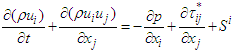
Interaction between an animal and its habitat is one of the crucial factors in the evolution process. In aquatic environments, marine species have developed some unique morphological features with hydrodynamic consequences to overcome necessity of life over the course of million years. In this paper, hydrodynamic effects of the longitudinal-dorsal ridges covering the upper-lateral sides of whale shark’s body as a prominent eidonomic characteristic of these species are studied with the aid of computational fluid dynamics (CFD). In this regard, flow physics of the problem is numerically simulated at high Reynolds number, i.e. 1.4×10⁷ corresponding to the swimming of a 10 meter-whale shark at its average speed, i.e. 5km / h, using Lam-Bremhorst turbulence model. The results indicate that presence of the longitudinal ridges leads to formation of streamwise vortices which delays flow separation on the body and modifies hydrodynamic characteristics of the whale shark swimming. At sideslip angles, flow simulation results show that the ridges noticeably contribute to the ‘sinking feeling’ of the animal. Furthermore, spectral analysis of the unsteady simulation results in start-up phase of the whale shark’s tail beating in a quiescent flow environment depict that these morphological features uniformize energy content of the vortical structures originating from the tail/caudal peduncle (not caudal fin) via suppressing of its energy peaks.
Keywords: Whale sharks, Ridges, Functional morphology, Locomotion, Hydrodynamics, CFD, Ichthyology, Bionics
Cite this paper: Arash Taheri , Hydrodynamic Impacts of Prominent Longitudinal Ridges on the ‘Whale Shark’ Swimming, Research in Zoology , Vol. 10 No. 1, 2020, pp. 18-30. doi: 10.5923/j.zoology.20201001.03.
Article Outline
1. Introduction
- Whale sharks (Rhincodon typus) are the largest fish in the world that slowly swim in tropical open waters including oceans, seas and gulfs (Fig. 1). Mexico [1], Australia [2] and Philippines [3] possess largest known populations of these highly migratory marine species, although they can be widely found in all regions with tropical waters with relatively high temperature like Taiwan [4] and Indonesia [5]. Persian Gulf (Khalij-e Fars) at the south of Iran with its warmest ocean water on the planet hosts numerous species of this amazing animal during summer and winter seasons in zones with depths greater than 40 m [6]. Whale sharks have evolved a perfect streamlined body possessing pairs of pectoral, pelvic and dorsal fins, as well as one anal and one vertical caudal fin (Fig. 2). As one can see in the eidonomy of the animal, undoubtedly the most pronounced feature of its morphology for any viewer could be presence of the prominent ridges on the upper part, i.e. lateral and dorsal sections, of the marine animal (Fig. 1, 2). Whale sharks are born with a total length of 55-64 cm; mature ones have a total length of greater than 6 and 8 meters for male and female species, respectively [7]. Maximum total length of these giant filter-feeding sharks can reach to 17-21.4 meters [7,8].In contrast to whales that are breath-holding animals and do not have a gill, sharks including whale sharks have a gill and take oxygen from water for metabolism. It is also interesting to mention that white spot and stripe checkerboard patterns on the skin of whale sharks (Fig. 1) is a unique sign of any individual whale shark specie, similar to fingerprints for human being. This characteristic can be adopted along with artificial intelligence techniques, e.g. pattern recognition methods, to identify whale shark individuals [2,9]. In this regard, photo of spot patterns in a window behind the whale shark’s gill (Fig. 1) is sufficient for a successful pattern recognition process [9].
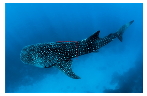 | Figure 1. Whale shark swimming in Indian Ocean [21]; red dashed line window: a zone typically adopted for identification of species [9] |
2. ‘Whale Shark’ Body Model
- To construct a 3D body model of a whale shark (Fig. 2), cross-sections of a 1:40 scaled-down whale shark model are scanned and digitalized in selected planes perpendicular to the longitudinal (z) axis. Then, a total number of 16 cross- section curves and 4 guide curves forming the external shape of the whale shark body (in the mid-planes defined by x=0 and y=0) are numerically generated by high resolution in MATLAB and imported to the SolidWorks CAD environment [23]. The final 3D numerical whale shark body model is majorly constructed by applying a lofting process, as shown in Fig. 2. The latter process is performed by stitching successive cross-section curves controlled by guide curves.
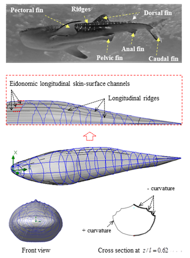 | Figure 2. Whale shark’s body morphology; Top: eidonomy (external morphology) details (modified from the base picture [22]), Middle-Bottom: a 3D biomimetic-scaled body model constructed in the present study, adopted for all upcoming CFD simulations |
3. Numerical Methodology
- To perform numerical flow simulations at a series of AoAs,
 and sideslip angle
  , the model is positioned at a fixed point in space and all above characterizing angles are implemented via freestream blowing angle with respect to the longitudinal z-axis (Fig. 3).
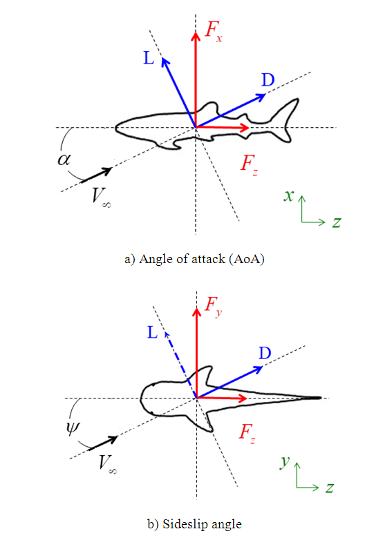 | Figure 3. Coordinate system adopted for ‘whale shark’ flow simulations |
 of the order of 107. In general, ‘whale sharks’ are among slow swimmers in oceans; as stated earlier these giants come to water surface for thermoregulation where a faster current exists about 2.5 m/s [24]. For instance, a ‘whale shark’ with a body length of 10 m that swims with a resultant speed of 5
  experiences fully turbulent flow over its body at
  . In this paper, all numerical simulations are performed at this Reynolds number. For simulations with imposing
  , inflow velocity is applied as below:
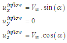 | (1) |
 , inflow is defined as below:
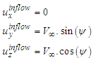 | (2) |
3.1. Computational Domain and Grid Generation
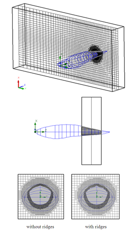
- Computational grids for numerical flow simulations are generated with the aid of SolidWorks meshing tools with capability of basic Cartesian mesh generation and applying an adaptive local grid filter to capture geometry of the ridges and boundary layers [25]. After performing grid convergence tests, a well-converged grid with 1.6 million elements is adopted here for all upcoming flow simulations. Fig. 4 and Fig. 5 show the computational mesh generated around the body model of a whale shark with ridges. It exhibits a well-resolved body-fitted mesh clustering to the wall to capture all details of the geometry. As shown at top of the figure, to minimize effects of the boundaries, the computational domain is extended about 3 and 4 times of the body length in x-y and z directions, respectively.
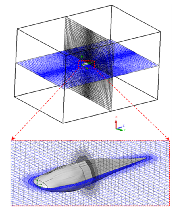 | Figure 4. Computational domain with an adaptive grid generation around the ‘whale shark’s body model |
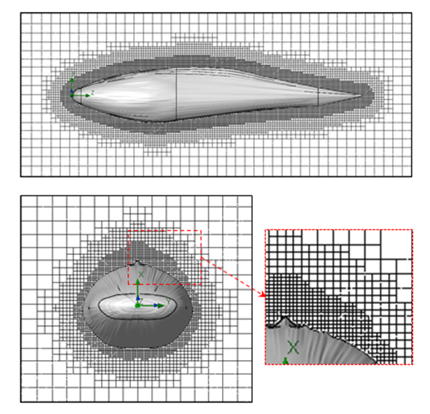 | Figure 5. Computational grids at cross-sections in the middle planes: side view (top) and front view (bottom) |
3.2. Turbulent Flow Treatment and Settings
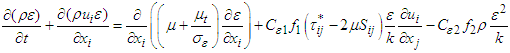
- Turbulent flow equations over the whale shark’s body model are solved at
 using unsteady Reynold averaged Navier-Stokes (URANS) technique [25]. In this regard, turbulence is treated with Lam- Bremhorst low- Reynolds number (LB LRN, hereafter)
  model using SolidWorks Flow Simulation (SFS) solver [25,26]. The name of ‘low-Reynolds number’ here should not be confusing; in fact this refers to ability of the aforementioned model to treat low-speed boundary layers. This is achieved by taking into account wall-distances and using at least 10 computational nodes in the boundary layer [25]. In general, governing equations of the problem before applying Reynolds triple-decomposition can be expressed in Einstein tensor notation as below [25]:
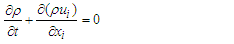 | (3) |
 | (4) |
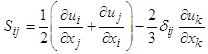
 and
and  , is defined as the following:
 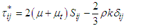 | (5) |
 | (6) |
 and
and  is turbulent eddy viscosity and kinetic energy, respectively, while
  denotes the Kronecker delta.
  and
and  equations are coupled as follows [25,26]:
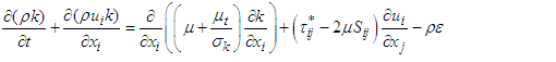 | (7) |
 | (8) |
 To calculate
  , one can use the following formula:
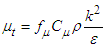 | (9) |
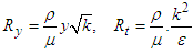
 and
and  and
and  are calculated as below:
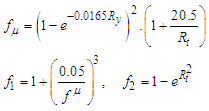 | (10) |
 | (11) |
 is the wall distance. Finally time and length scales are computed as below [27]:
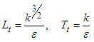 | (12) |
 and
and  forces acting on the whale shark’s body by its interaction with the flow field are continuously monitored to ensure satisfaction of all convergence criteria. These measures are automatically applied by SFS solver based on dispersion of goal functions which leads to lowest residual errors [23].
 4. Results and Discussion
- In this section, results of numerical simulations of turbulent flows over the whale shark’s body model are presented at
 . Validity of the numerical simulation strategy was confirmed in the previous study [20] by performing flow simulations over an ellipsoid at zero AoA and comparing drag coefficient with the experiment,
  . It was shown that applying an averaged roughness of 10 microns results in a good match to the experiment [20].
4.1. Effects of Ridges in Streamwise Swimming
- In this subsection, streamwise swimming of the ‘whale shark’ at
 is considered. Fig. 6 shows convergence history of the vertical and axial forces. It is interesting to notice that presence of the prominent ridges on the whale shark’s geometry and geometrical difference between top
  and bottom
  sections in the side-view profile of the animal (Fig. 7) breaks symmetry of the flow field. As one can see in Fig. 6, negative Fx is generated at
  , which means whale shark’s eidonomic shape generates a force opposite to the buoyancy or in the direction of the animal weight force. This feature also helps in what is so-called ‘sinking feeling’ of whale sharks, in accordance with experimental observations reported by Gleiss et al [28]. It is worth to mention that sharks do not have a ‘swim bladder’ like other fishes or Blubber fat layer under their skin like cetaceans or whales to facilitate their floating in water; instead their oily liver consists of oil/fats lighter than water that partially helps them to be afloat, but it is not enough and sharks have to swim continuously to avoid sinking. Gleiss et al. used a tagging technique to study movement strategies of whale sharks by recording some physical and environmental parameters. They observed that whale sharks take advantage of their negative buoyancy for gliding through descent movements from surface to the depths [28]. In another study, Gleiss et al. showed that negative buoyancy can be more efficient in the shark’s accelerated movements [29].
 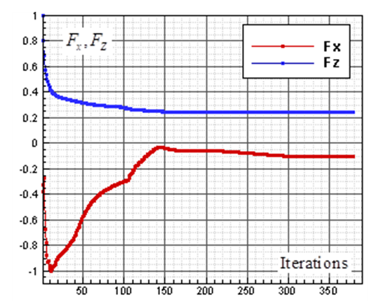 | Figure 6. Convergence history of the normalized vertical and axial forces acting on the whale shark’s body model at  |
 is generated, thanks to the streamlined profile of the body and presence of the prominent ridges.
 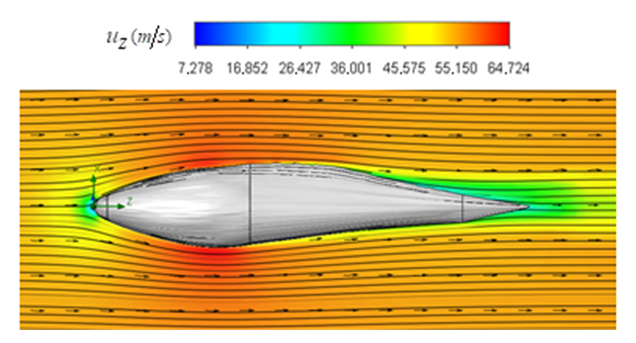 | Figure 7. Axial velocity field around the whale shark’s body at  in the middle plane defined as y=0 in the middle plane defined as y=0 |
 -criterion with a threshold defined as
  can be utilized [30]. Practically, an appropriate value of the threshold level is case-dependent. Fig. 8 represents hidden structures generated on the whale shark’s body model extracted by
  . As one can see in the figure, streamwise vortices are generated by special topology of the prominent ridges on the whale shark’s body. It can be postulated that presence of these streamwise vortices injects some extra momentum from higher velocity region into the near-body zone with lower velocity and suppresses or delays separation.
 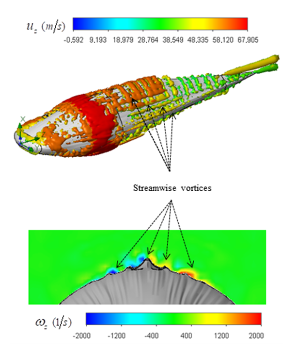 | Figure 8. Vortical structures/shear layers developed on the whale shark’s body model captured by  -criterion at -criterion at  , isometric view (top); streamwise vorticity generated by the prominent ridges on the whale shark’s body model (bottom) , isometric view (top); streamwise vorticity generated by the prominent ridges on the whale shark’s body model (bottom) |
4.2. Effects of Ridges in AoA
- As mentioned before, whale sharks are gentle swimmers with not relatively high physical activities in oceans and their swimming speed can be considered 5
 in average and can ultimately reaches to 13
 over a short period of time as reported by Hsu et al. [4]. This range of speeds in combination with ocean current speeds having maximum value of 2.5
 near the surface creates a broad range of AoAs and sideslip angles. This is important to be considered because whale sharks spend a relatively large period of time near the ocean surface for thermoregulation. In this subsection, turbulent flows over the whale shark’s body are simulated at
 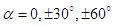 and
and  . Fig. 9 shows variation of lift and drag coefficients of the whale shark’s body versus AoA for all performed numerical simulations in this subsection. As one can see in the figure, symmetry breaks for positive and negative AoA counterparts; although similarity exists between two cases. It is worth to mention that drag and lift coefficients are calculated here based on the body’s planform area. In the literature, experimental drag coefficient data for a 3D streamlined body is equal to 0.04 based on frontal area for
  at
at  [31]; considering geometry of whale shark’s body and using planform area, instead of frontal area, drag coefficient is calculated as 0.014. Simulation results show that drag coefficient is augmented to 0.015 calculated based on the planform area at
  , due to an increase in the wetted area.
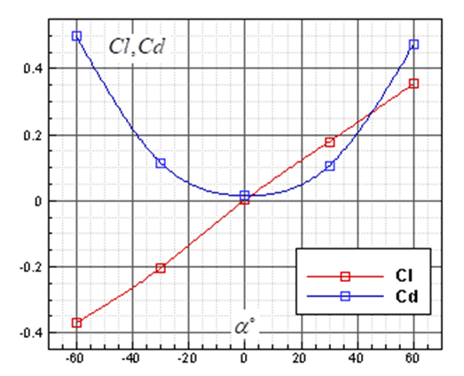 | Figure 9. Life and drag coefficients based on planform area generated by the whale shark’s body model at different AoAs at  |
 and
and  , respectively. By comparing of these figures, it is clear that absolute values of the converged values of vertical and axial forces increase by increasing AoA.
 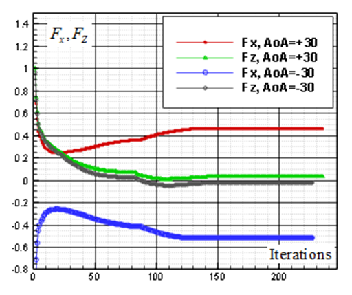 | Figure 10. Convergence history of the normalized vertical and axial forces acting on the whale shark’s body model at  |
 | Figure 11. Convergence history of the normalized vertical and axial forces acting on the whale shark’s body model at  |
 cases no longer exist; in
  , there exists a heavier wake and a wider bundled pathlines compared to
  . Presence of ridges on the dorsal and lateral sides of the animal majorly modifies topology of the flow fields. For
  cases, the abovementioned effect is present but less pronounced.
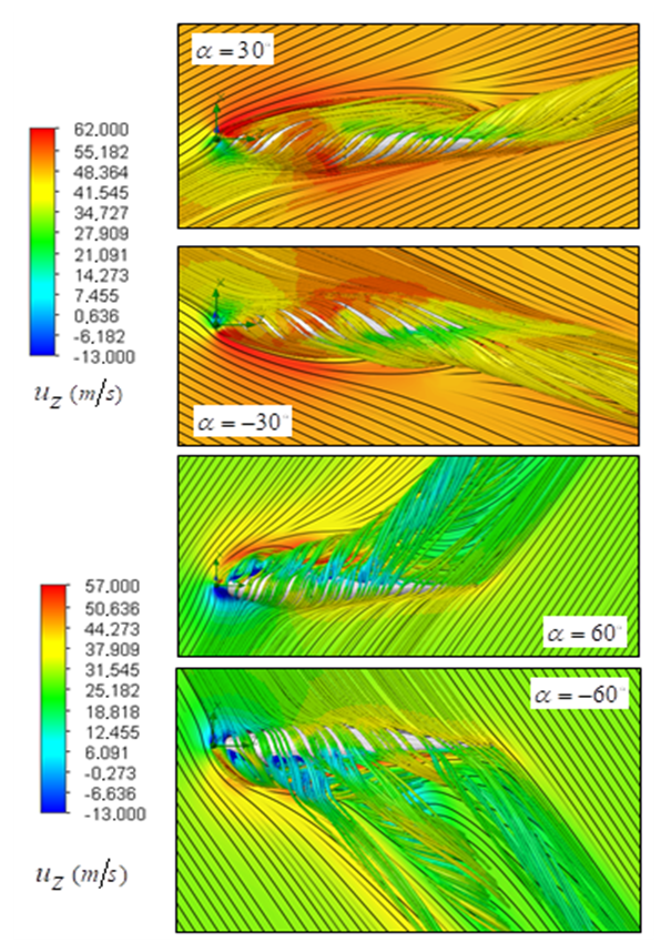 | Figure 12. 3D pathlines over the whale shark’s body model along with axial velocity fields at different AoAs in the middle plane defined as y=0 |
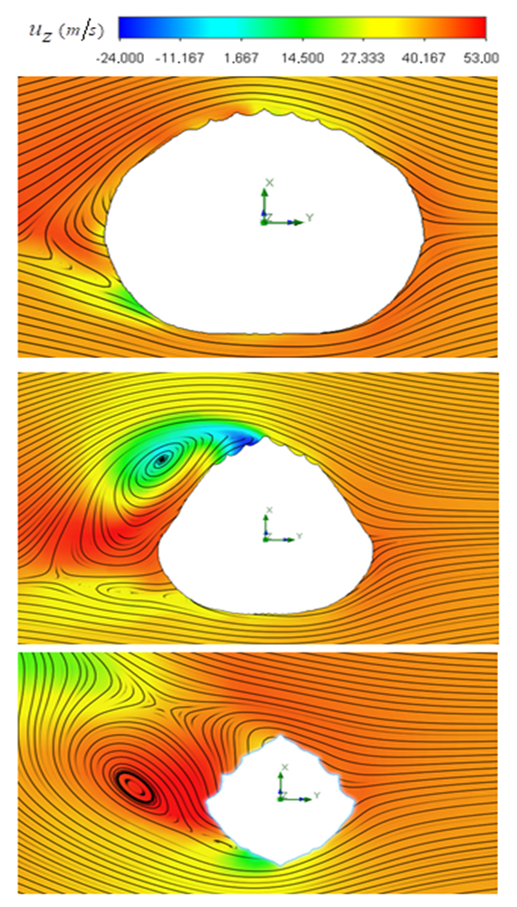
 . As one can see in the figure, two dominant counter-rotating vortices are generated on top of the whale shark’s body. These vortical structures lead to formation of regions with high and low axial velocities close together on top of the body, as shown in the figure. It is interesting that these rotating regions are detached from the whale shark’s body in a way that two saddle-points are clearly formed in the pathlines map.
 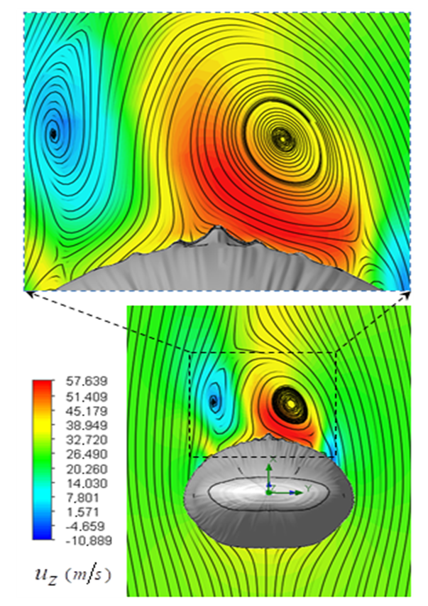 | Figure 13. Mean axial velocity field around the whale shark’s body at  in the middle plane at z/L=0.5, where (L) denotes the body length; pathlines close to the body (top), front view field (bottom) in the middle plane at z/L=0.5, where (L) denotes the body length; pathlines close to the body (top), front view field (bottom) |
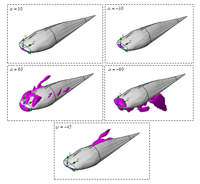
 -criterion. Fig. 14 depicts vortical structures developed on the whole body of the whale shark. As can be expected and shown in the figure, different 3D patterns of vortical structure developments exist at different AoAs. As depicted in the figure, structures start to be shaped from the animal’s nose at all AoAs. For positive angles, structures are more pronounced on the top of the whale shark’s body, while for the negative angles, structures are more dominant on the bottom part of the body. At
  , two distinct tail-like vortical structures attached to the whale shark’s body corresponding to vortex cores with minimum pressure are generated extending downstream with a slope angle equals to the imposed AoA. By increasing of AoA to
  , more vortical/ shear layer structures are generated on the body as expected apriori. As it is visible in the figure, at
  detached coherent structures are also captured by
  -criterion which can be linked with strength of the aforementioned structures and the threshold values; in general by increasing absolute value of
  , fewer structures with higher strength are captured. By comparing
  cases, it is observed that at negative AoA concentration of the flow structures with strong rotation centers decreases compared to the positive AoA, this fact is also visible in the 3D pathlines embracing the body illustrated in Fig. 14. As one can also conclude, due to presence of the prominent longitudinal ridges and dissymmetry which basically exists between the top and bottom of the whale shark’s body profile, vortical structures generated on the body should be different, although similar.
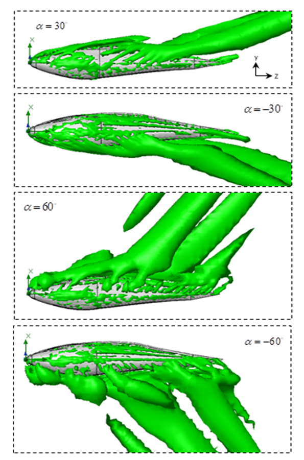 | Figure 14. Vortical/shear layer structures developed on the whale shark’s body model at different AoA, extracted with  |
4.3. Effects of Ridges in Sideslip Angles
- As mentioned before, whale sharks experience sideslip angles while swimming, majorly induced by surface currents and whale shark’s gentle activities. In this subsection, at a relatively high sideslip angle,
 , turbulent flow over the whale shark’s body model is numerically simulated at
  . Fig. 15 shows convergence history of the normalized forces acting on the whale shark’s body by passing turbulent flow at the sideslip angle. As one can see in the figure, due to presence of ridges on the dorsal-lateral parts of the body and geometrical dissymmetry of the eidonomic shape of whale sharks in the vertical direction (x-axis), negative Fx is majorly generated (opposite to buoyancy force), which profoundly contributes to the ‘sinking feeling’.
 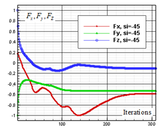 | Figure 15. Convergence history of the normalized vertical, lateral and axial forces acting on the whale shark’s body model at  |
 sideslip angle. As shown in the figure, a dominant vortical structure corresponding to a strong vortex core is majorly generated on the left-side of the body (i.e., downstream) originating from the body mid-section. Although, a smaller vortical structure is also present at the aft zone of the whale shark’s body at this sideslip angle. Some non-coherent vortical structures with sparse distribution are captured on the right-side of the body.
 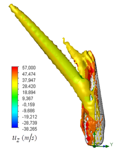 | Figure 16. Vortical/shear layer structures developed on the whale shark’s body model at sideslip angle  captured by captured by  |
 | Figure 17. Mean axial velocity field around the whale shark superimposed with flow pathlines at  in the vertical planes defined from top to bottom as z/L= 0.3, 0.5 and 0.8; where (L) denotes the body length in the vertical planes defined from top to bottom as z/L= 0.3, 0.5 and 0.8; where (L) denotes the body length |
4.4. Predicted Separation Zones
- Fig. 18 illustrates the mean flow separartion zones defined as iso-surfaces of reverse flows obtained from turbulent flow simulations over the whale shark’s body.
 | Figure 18. Separation zones formed on the whale shark’s body model at different AoA and sideslip |
 , separation zones are only limited to the nose of the marine animal. By increasing AoA to
  , separation zones are visible at whale shark’s nose for both angles; non-coherent sparse separation zones are majorly generated on top and bottom of the body at positive and negative AoA, respectively. At the sideslip angle, relatively small separation zone forms on the left side of the whale shark’s body.
 4.5. Effects of Ridges on Tail Beating Hydrodynamics
- Whale sharks use undulatory/oscillatory movements of their aft-body/ tail (typically exceeding caudal peduncle zone) and large vertical caudal fin from side to side for propulsion generation. Their caudal fin size from its top-tip to the bottom-tip is about 1/3 of their total body length. To have an idea how presence of the prominent ridges modifies hydrodynamics of the tail-beating, here an unsteady simulation of start-up phase of the whale shark’s tail beating in a quiescent flow environment is considered. Fig. 19 illustrates a simplified model of the problem. It is assumed in the model: by tail beating, whale sharks move aft-part of the body/tail and caudal fin in a rotation with a constant frequency about a pivot point forming an arm with a length equals to a given percentage of the body length. In the model, by tail beating a linear velocity distribution is generated as
 ; where R is length of the arm and
  is the angular velocity of the tail beating. One can rewrite the above equation as
  ; where
  is a local arm length variable defined at any point on the tail and
  is the position of the assumed pivot point on the body.
 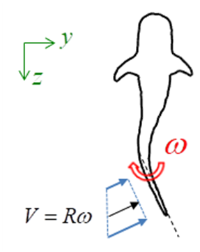 | Figure 19. A simplified model for start-up tail beating of a ‘whale shark’ in a quiescent flow environment |
 .
. | Figure 20. Computational domain and grid generation around the whale shark’s tail with/without ridges |
 . Meekan et al. reported frequency and amplitude of the tail beating of two 4 and 7 meter whale sharks, which represents a linear variation between modal frequency and amplitude of the whale shark tail beating for propulsive strokes [11]. For unsteady simulations in this subsection,
  is applied. Fig. 21 shows mean lateral velocity fields and pathlines over the whale shark’s tail with/without ridges at z/L= 0.75 obtained from the time-dependent simulations. As one can see in the average field, presence of the ridges profoundly modifies topology of the flow field and formation of vortical structures around the tail. Thus the generated von Kármán vortex street are majorly modified by these ridges.
 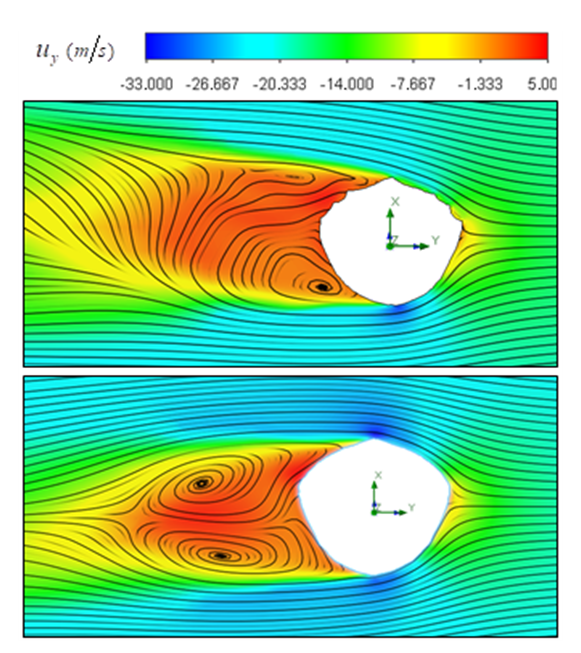 | Figure 21. Mean lateral velocity field and pathlines over the whale shark’s tail at z/L= 0.75; where (L) denotes the body length; with ridges (top), without ridges (bottom) |
 ) and vortical structures formed in the tail beating. As shown in the figure, some strong vortex cores are captured by
  in a reference frame positioned on the whale shark’s tail. The figure shows that presence of the ridges modifies details and global features of the flow fields.
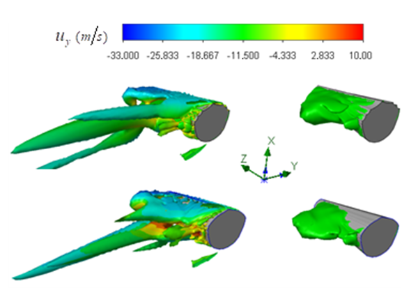 | Figure 22. Mean vortical structures developed on the whale shark’s tail (left); separation zones (right): with (top) /without (bottom) ridges |
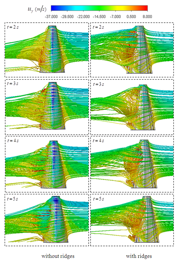 | Figure 23. Unsteady 3D pathlines in the start-up phase of a whale shark’s tail beating in a quiescent flow with ridges (right) and without ridges (left) |
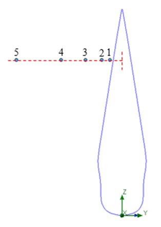 | Figure 24. Probe points adopted for lateral velocity signal sampling |
|
 for a total physical-time duration of
  . In this regard, sampling process was started after passage of
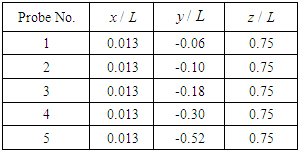
  start-up phase spent to achieve a statistical convergence state. As one can see in the figure, for all probe points presence of the ridges makes the energy curves more uniform via suppressing of the positive/negative peaks of the curves; in this way ridges behave as an efficient energy damper for vortical structures originating from caudal peduncle zone. In this way, large vortical structures with maximum energy (marked by dashed-circles in Fig. 25) are effectively removed by the ridges. As one can also see in the figure, only dominant unsteadiness in the flow field can ultimately be seen in URANS technique as adopted in this paper. To further investigate effects of the ridges on turbulent eddies and reproduce turbulence spectrum in full with -5/3 decay in the inertial subrange, full/semi- resolving techniques like DNS, LES or DDES should be utilized in future to resolve eddies, although by spending more computational costs.
 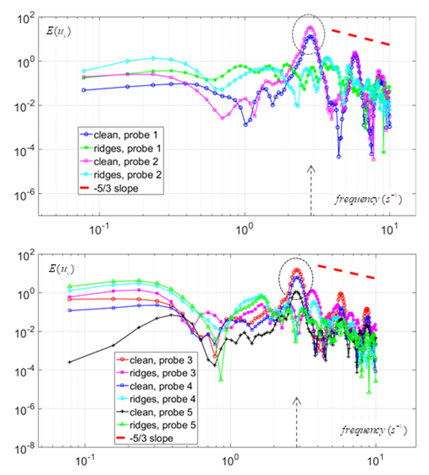 | Figure 25. PSD of the lateral velocity signals captured by probes (Table 1) in the tail/caudal peduncle region of a whale shark |
5. Conclusions
- This paper shed some light on the hydrodynamic effects of the prominent ridges as an eidonomic feature on locomotion of the largest known fish on the planet. It was discussed that each two successive neighbour ridges with its special geometry create a so-called ‘fluid flow channel’ on the whale shark’s skin; these 6 diverging-converging channels with variable depths in the longitudinal direction act as a bionic structure for generation of streamwise vortices. These vortices in turn minimize formation of the separation zones. Numerical simulations in the streamwise swimming also showed that, a downward force (opposite to the buoyancy) is generated although small, by the external shape of the whale shark which contributes to the so-called ‘sinking feeling’. Especially at swimming with sideslip angle, a noticeable amount of force acting on the whale shark body is generated by the ridges in the direction opposite to the buoyancy, which clearly contributes to the ‘sinking feeling’. This geometry-induced negative-buoyancy feature along with the default negative-buoyancy of sharks can be potentially used by whale sharks for very fast diving to the depths. As simulations show, this can be simply performed by adjustment of the whale shark’s heading with a sideslip angle while swimming. Numerical simulations at different AoA and sideslip showed that presence of ridges considerably modifies flow structures formed in the flow field. Thanks to streamlined body shape of the whale sharks and presence of the prominent ridges on their body, flow separations are limited to small zones on the body.Unsteady simulations of whale shark’s tail beating model showed that presence of ridges radically modifies characteristics of vortical structures originating from the caudal peduncle zone. PSD analysis showed that energy content of the dominant vortical structures is noticeably modified by the ridges and peaks of the energy curves are suppressed. In this view, the ridges act as bionic energy dampers for vortical structures originating from the caudal peduncle zone.
ACKNOWLEDGEMENTS
- The author would like to sincerely acknowledge every single effort done by institutes, organizations and individuals to protect ‘whale sharks’ worldwide.