-
Paper Information
- Paper Submission
-
Journal Information
- About This Journal
- Editorial Board
- Current Issue
- Archive
- Author Guidelines
- Contact Us
International Journal of Statistics and Applications
p-ISSN: 2168-5193 e-ISSN: 2168-5215
2026; 16(2): 52-60
doi:10.5923/j.statistics.20261602.02
Received: Aug. 20, 2026; Accepted: Sep. 8, 2026; Published: Sep. 11, 2026

A Survey-Weighted Model-Assisted Framework for Indirect Under-Five Mortality Estimation from Summary Birth Histories
 Abstract
 Reference
 Full-Text PDF
 Full-text HTML
Samuel O. Adeyemo, Emmanuel U. Ohaegbulam, Felix N. Nwobi
Department of Statistics, Imo State University, Owerri, Imo State, Nigeria
Correspondence to: Samuel O. Adeyemo, Department of Statistics, Imo State University, Owerri, Imo State, Nigeria.
| Email: |  |
Copyright © 2026 The Author(s). Published by Scientific & Academic Publishing.
This work is licensed under the Creative Commons Attribution International License (CC BY).
http://creativecommons.org/licenses/by/4.0/

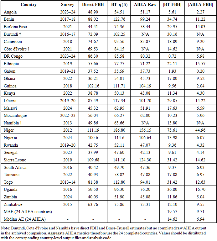
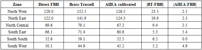
Classical indirect estimation relies on Summary Birth Histories (SBH) where civil registration or full birth histories are unavailable, but Brass-type procedures pool maternal-age-group data before applying model-life-table transformations. In non-homogeneous populations, this ordering can provide a mix of fertility composition and mortality risk. This paper develops An Improved Indirect Estimation Approach (AIIEA), a survey-weighted, model-assisted approach that consists of a quasibinomial conditional mortality surface  , followed by birth-weighted design aggregation (A) and ratio-preserving benchmark calibration (C). The framework formalizes non-identifiability of exact period under-five mortality from SBH, mixture distortion, non-commutativity, compositional bounds, and calibration preservation. In the Nigeria DHS 2023-24 internal application, calibrated AIIEA estimates had a zonal mean absolute discrepancy of 2.94 deaths per 1,000 relative to direct full birth history estimates, compared with 11.64 for Brass-Trussell Manual X, a 74.7% reduction interpreted as within-sample subnational reconciliation rather than out-of-sample prediction. In the 24 comparable country applications within a 27-country DHS archive, national MAE was 9.71 per 1,000 for raw AIIEA and 19.57 for the classical comparator. AIIEA extends, rather than rejects, the Brass tradition by making conditioning, survey design and calibration explicit.
Keywords: Under-five mortality, Summary birth history, Indirect estimation, Brass-Trussell, Model-assisted survey estimation, Quasibinomial regression, Calibration, Nigeria DHS, AIIEA
Cite this paper: Samuel O. Adeyemo, Emmanuel U. Ohaegbulam, Felix N. Nwobi, A Survey-Weighted Model-Assisted Framework for Indirect Under-Five Mortality Estimation from Summary Birth Histories, International Journal of Statistics and Applications, Vol. 16 No. 2, 2026, pp. 52-60. doi: 10.5923/j.statistics.20261602.02.
Article Outline
1. Introduction
- Under-five mortality, denoted
 , is the probability that a live-born child dies before exact age five. It is a key demographic and public health indicator as it serves as an indicator of child survival, maternal health, childhood disease, nutrition, household welfare, health system performance and social inequality. Where the civil registration and vital statistics systems are adequate and complete,
  can be estimated directly from registered births and deaths data. In many low- and middle-income settings, however, the estimation of mortality remains largely based on the household surveys and censuses. [1], [2]There are two survey data structures that are prevalent in the estimation of child mortality. Full birth histories record child-level dates of birth, survival status and age or date at death. They permit direct life-table estimation, but are lengthy, and may be associated with recall displacement, age-at-death heaping, omission and high sampling variance when broken down into small domains. Summary birth histories collect only the number of children ever born and the number surviving or deceased for each woman. In censuses and compact surveys, they are shorter and more feasible, but sacrifice the timing information that allows for the identification of period mortality, without the use of auxiliary assumptions. The classical solution to the SBH problem is the Brass tradition and its several modifications (by Sullivan, Trussell, Manual X, Feeney, Zlotnik-Hill, QFIVE, MORTPAK and other related demographic tool). These techniques convert maternal-age-group proportions dead into probabilities of dying before selected childhood ages using multipliers derived from model fertility and mortality schedules. The limitation addressed here is that these procedures typically pool heterogeneous women prior to transformation. [3], [4], [5], [6], [7], [8], [9], [10], [11]However, in such a context as Nigeria, where fertility, educational attainment, wealth, residence and regional mortality risks differ sharply, pooling before conditioning can confound mortality risk with population composition. [12], [13], [14]This paper develops the methodological foundations of AIIEA. The three-point idea is to condition, aggregate, calibrate. The paper is as a contribution to mathematical demography and applied survey statistics. It formalizes the reason why exact period
  cannot be identified with SBH, defines the estimand that is compatible with SBH, derives the operator framework for AIIEA, and demonstrates its empirical behavior using Nigeria DHS 2023-24.
2. Classical Indirect Estimation and the Estimation Problem
- Direct full birth history estimation uses interval survival probabilities to obtain under-five mortality. If
 denotes the probability of dying in standard age interval x below exact age five, then [2]
 | (1) |
 denote the number of children woman j has ever born, and, let
  denote the number of children woman j has survived and
  the number of children woman j has lost. The reported proportion dead (RPD) for the women was [4], [11]
 | (2) |
 | (3) |
 | (4) |
 is a multiplier dependent on the assumptions in the fertility and mortality schedules. The multipliers are given in Trussell and Manual X in terms of parity ratios, typically of the form [7], [8]
 | (5) |
3. Estimand Hierarchy and Age-Time Interpretation
- AIIEA begins by separating three objects that are often blurred in applied mortality estimation: the ideal period target
 , the functional target
  that is compatible with the SBH, and the calibrated operational target
  . The time periods
  requires deaths and exposures for each child age and time period. SBH only gives information on cumulative births and survivorship outcomes reported by women at the time of the survey. The information gap is not just a computational gap but a structural gap.AIIEA will therefore interpret the raw estimate as an SBH compatible mortality functional. A convenient representation uses an age-time exposure kernel:
 | (6) |
 is the mortality surface by child age a and retrospective time t in domain d, while
  is the exposure-density kernel induced by fertility timing, child age, survival reporting and maternal age group g. Younger maternal age groups generate more recent and concentrated kernels, while older age groups generate more diffuse retrospective kernels. This motivates the primary empirical age window of women aged 20-34.
4. AIIEA as an Operator Framework
- AIIEA is represented as a three-stage composite operator:
 | (7) |
4.1. Stage 1: Survey-Weighted Quasibinomial Conditional Surface
- For woman j with
 AIIEA models the conditional expected number of reported child deaths as
 | (8) |
 | (9) |
 | (10) |
4.2. Stage 2: Birth-Weighted Design Aggregation
- After estimating
 individual fitted risks are obtained as
 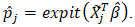 For domain d, the raw AIIEA functional is the birth-weighted Hájek design ratio [17], [18], [19]
 | (11) |
4.3. Stage 3: Benchmark Calibration
- Let
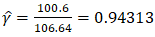
 be a defensible national benchmark, such as a direct FBH estimate from the same survey or an official national series. The calibration scalar is [19]
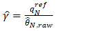 | (12) |
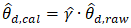 | (13) |
5. Formal Properties
5.1. Non-Identifiability of Exact Period Mortality from SBH
- Without auxiliary assumptions, exact period
 is not uniquely determined by the child dates of birth and the dates of child–human exposure, if these are unobserved. The same values for
  and
and  can be produced by different combinations of fertility and mortality history. Hence AIIEA does not claim to calculate the exact period mortality from SBH. It is an estimation of an SBH-compatible function followed by calibration to a benchmark.
5.2. Mixture-Distortion Decomposition
- Suppose domains d and e contain R strata with birth shares
 and
and  and stratum-specific mortality summaries
  and
and  The pooled difference decomposes as
 | (14) |
5.3. Non-Commutativity of Pooling and Transformation
- Let
 be an indirect transformation depending on a pooled proportion P and demographic parameters z, such as parity ratios or model-life-table coefficients. If
  is nonlinear in P, or if z changes with the composition used to form the pooled statistic, then pooling and transformation generally do not commute:
 | (15) |
5.4. Compositional Distortion Bound
- The compositional term in Equation (14) satisfies the bound
 | (16) |
 mean that
  will be at most times less than 1, but the same is not true for the distance between the probability vectors
  which can be as large as 2. The bound connects demographic intuition of compositional heterogeneity with a formal distance between the vectors of birth-shares of the subgroups.
5.5. Calibration Preservation
- The calibration operator preserves national alignment, ratios and rank ordering. Because National alignment follows because
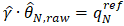 . Ratio preservation follows because
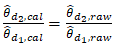 | (17) |
 is positive, rank preservation follows immediately. Also under common multiplicative discrepancy, calibration scale-invariance means that if raw estimates are on a common scale which is a multiple of the domain functional, then on the calibrated scale domain estimates get the benchmark-scaled estimates. Calibration does not address domain-specific bias, it does only address a common national scale discrepancy.
6. Estimation of Variance and Asymptotic Justifications
- Under complex sampling, the survey-weighted quasibinomial estimator is considered to be a pseudo-likelihood or quasi-score estimator. Under standard regularity conditions for survey M-estimation, [18], [19]
 | (18) |
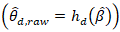 is
is | (19) |
 | (20) |
 is itself estimated rather than treated as fixed, its uncertainty should also enter the final variance. A first-order extension may be written as
  approximately equal to the gradient contribution from
 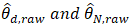 plus the contribution from
  including covariance terms where the benchmark and AIIEA raw estimates are estimated from the same survey. In the present internal Nigeria comparison, the benchmark is used primarily to define the calibration scale; the point-estimate validation is therefore interpreted at the zonal level rather than as evidence of zero national error.
7. Empirical Application: Nigeria DHS 2023-24
- The official Nigeria DHS 2023-24 Individual Recode (IR) microdata is used for the empirical illustration. The primary analytical sample consists of 13,739 women age 20-34 who had at least one child ever born and had no missing model or survey design variables. The v201 variable is used to measure the number of children born,
 to report on deaths of children,
  to measure the sampling weight, v001 to measure the primary sampling unit, and
  as defined in the release to report on the stratification variables supplied. The design-weighted sample comprises of 43,575.1 children ever born and 4,646.8 reported child deaths; the SBH proportion-dead statistic (unmodelled by design) has DEFF = 74.60. Maternal age group, geopolitical zone, urban-rural residence, maternal education and household wealth are included as conditional factors. The internal national calibration anchor for the within-survey direct FBH estimate is a FBH estimate corresponding to the dated birth histories of 100.6 deaths per 1,000 (Table 1). The classical indirect comparator is the Brass-Trussell Manual X. All reported estimates must be generated from the archived survey design object and analysis script and derived output tables. [20], [21]
|

|

 | (21) |
|
|

8. Sensitivity, Manual Computability and Portability
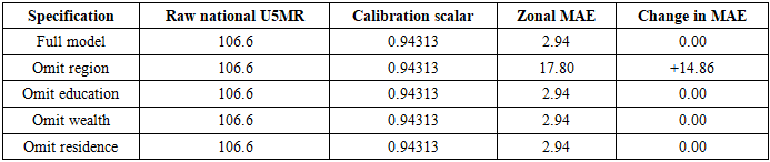
- The AIIEA was evaluated using age window sensitivity and covariate block omission. The preferred 20-34 window produced the lowest within-sample zonal MAE among the tested alternatives. This pattern is consistent with the timing-kernel argument that very young maternal ages provide limited exposure while older ages introduce more temporally diffuse exposure; it is not, by itself, an external test of predictive performance.The 20-34 restriction is therefore a primary analytical window rather than a claim that women aged 15-19 or 35-49 are irrelevant. In full operational use, analysts may report supplementary estimates for wider maternal-age windows or develop age-group-specific calibration strategies. The present paper reports the restriction transparently because the aim is to evaluate the most temporally interpretable SBH functional rather than to force all reproductive ages into a single period-like estimate.
|

|
|

9. Discussion
- The results are consistent with the theoretical explanation that the order of operation is important. In classical approaches, the pooling is often done prior to demographic transformations, while AIIEA conditions first, aggregates second, and calibrates third. Conditional on the presence of a pooled birth-share structure, conditioning prior to aggregation ensures that the observed spatial structure is maintained, but should it be present in a heterogeneous population. The Nigeria results are an example of this mechanism and the 24 country applications completed are a wider portability check.The Nigeria application shows close within-sample alignment with direct FBH at the zonal level while retaining the data economy of SBH. This agreement should not be interpreted as out-of-sample prediction because zone enters the fitted conditional surface. AIIEA also cannot recover exact child-level timing and remains dependent on reporting quality, model specification and calibration benchmarks. Its more specific contribution is a survey-weighted, model-assisted and auditable use of SBH microdata that retains observed heterogeneity until the aggregation stage.This method is not intended to replace the direct FBH estimation, the Bayesian small area estimation or the modelling performed by IGME official. When there is a history of a child or sample sizes are adequate, direct FBH is useful. The smoothing of spatial and temporal variation is still possible with the Bayesian approach, as well as with the small-area approach. AIIEA is filling a different void: in situations where only summary histories are available, or subnational SBH estimates are required as an operational monitoring tool. [22], [23], [24], [25]
9.1. Relationship to the Brass Tradition
- This proposed estimator is not meant to be a criticism of Brass, Sullivan, Trussell and Manual X. These techniques addressed a long-standing problem, that of estimating childhood mortality from a limited amount of fertility and survivorship data when event histories are not available. Their ongoing contribution comes from their demographic parsimony and transparency. When the analyst has both respondent-level SBH microdata and sampling weights, but not all child-level timing, AIIEA asks if the classical order of operations is still sufficient.The classical estimator begins with a maternal-age group i, forms the pooled proportion dead Pᵢ, and then applies a multiplier kᵢ. In a homogeneous population this is sensible. In a heterogeneous population, however, the pooled Pᵢ is already a mixture of fertility composition and mortality experience. AIIEA therefore keeps the Brass insight that SBH can be transformed into childhood mortality information, but changes the timing of the transformation: it conditions on heterogeneity before aggregating.
9.2. Interpretation of the SBH Functional
- One of the criticisms of indirect estimation is that the resulting estimate might be a period mortality rate when no actual period exposure exists in the SBH data. AIIEA's solution is to break down the ideal demographic target from the identifiable SBH functional. The raw AIIEA estimator is an SBH-compatible mortality functional summarizing the reported risk of child-death over the retrospective exposure kernel of the process of fertility timing and maternal age composition. Calibration then maps this raw functional onto a benchmark-aligned scale.
9.3. Quasibinomial Working-Mean Specification
- The quasibinomial model is used since the response is number of child deaths out of children ever born for each woman. If the outcome of child deaths was a simple binomial conditional on the woman's set of covariates, child-death outcomes in a woman's birth history would be independent Bernoulli trials with variance
 . That assumption is too narrow for demographic survey data. Children born to the same woman share maternal characteristics, household circumstances, community risk, period conditions and reporting mechanisms. The quasibinomial variance is an overdispersion scale φ, which does not need to be the binomial variance but allows the mean model to be logistic. [15], [16]
9.4. Survey Design as Part of the Estimator
- AIIEA treats complex survey design as part of the estimator rather than as an optional post-estimation correction. DHS surveys use stratification, clustering and unequal selection probabilities. Failure to account for these features can lead to biased point estimates and uncertainty estimates, especially for subnational mortality outcomes where cluster composition is strongly related to geography and socioeconomic conditions. The survey weight
 enters both the quasi-score equations and the aggregation operator. The primary sampling unit and stratum enter the sandwich covariance estimation. [18], [21]
9.5. Relationship to Bayesian Small-Area Models
- AIIEA should be distinguished from Bayesian small-area mortality models. The goal of the Bayesian approaches is to borrow strength across the areas, to quantify the uncertainty hierarchically and to stabilize the sparse estimates of the direct ones. AIIEA addresses a different problem: how to extract more defensible indirect estimates from SBH microdata before aggregation. It does not require spatial priors, adjacency matrices or time-series smoothing, although it can complement Bayesian models by producing improved SBH-based inputs or diagnostics. [22]-[25]
10. Limitations
- First, AIIEA is constrained by the reporting error inherent in SBH, such as the lack of reporting for children who have died and problems with recalling children's ages. Second, the quasibinomial specification is a working mean model rather than a full generative mortality process. Third, a national benchmark must be defensible in order for it to be used in calibration. Fourth, the Nigeria zonal comparison is internal: geopolitical zone enters Stage 1 and the same six zones define the validation criterion. The 74.7% reduction therefore measures within-sample reconciliation, not out-of-sample predictive accuracy. Fifth, direct FBH comparators are themselves subject to recall and sampling error. Sixth, the multi-country archive contains 27 countries but only 24 completed raw AIIEA outputs; the remaining three are transparently marked in Appendix Table A1. Finally, observed covariates cannot remove unobserved heterogeneity, and uncertainty in the benchmark should be propagated when the benchmark is estimated rather than fixed. [3], [4]
11. Conclusions
- In this paper, AIIEA is proposed as a survey-weighted, model-assisted framework for indirect under-five mortality estimation from summary birth histories. The method extends the Brass tradition further by conditioning on observed heterogeneity prior to birth-weighted aggregation and applying transparent, ratio-preserving calibration only after the raw domain structure is estimated. The Nigeria DHS 2023-24 application exhibits substantially closer within-sample zonal reconciliation with direct FBH than Brass-Trussell Manual X, while the sensitivity analysis shows that this gain is driven mainly by explicit geographic conditioning. Also, across the 24 completed country applications in the 27-country archive, and when comparing the raw AIIEA to the classical comparator, the national absolute discrepancy is lower. These results provide an empirical basis for the proposition that AIIEA has potential as an extension of indirect estimation, and are illuminated by a mathematically explicit treatment of the method, but suggest that there is room for further research on out-of-sample validation, completion of the remaining country runs, and propagation of uncertainty of the benchmark.
ACKNOWLEDGEMENTS
- The authors wish to acknowledge the Demographic and Health Survey (dhsprogram.com) for approving and releasing the dataset used in this study.
DISCLOSURE
- Data Availability StatementThe DHS datasets used in the current study were accessed from the DHS Program repository (https://dhsprogram.com) by registering and approving for research purposes. The author can provide derived tables and code on reasonable request, with restriction on data use by DHS.FundingThis study received no external support.Conflict of InterestThe author has no competing financial interests and no competing non-financial interests to declare.Ethics StatementSecondary, anonymized DHS microdata is used in this study. Ethical approval for DHS survey protocols is obtained by the national ethics authorities and by ICF Institutional Review Board procedures. The author did not collect any primary data.
Appendix A. Multi-Country Portability Archive
- Appendix Table A1 reports the country-level direct FBH, Brass-Trussell and raw AIIEA comparisons. Direct FBH and Brass-Trussell results are available for all 27 archived countries. Raw AIIEA outputs are complete for 24 countries; dagger-marked rows are excluded from AIIEA summary metrics.
|