1. Introduction

Magnitude squared coherence and time lag analysis are employed within a variety of disciplines to provide insight and understanding of inter-related physical phenomena. These tools are most useful in relation to evaluation of time- and spatially-varying effects, especially for correlation of events which are changing with time in a broad band manner, as they are separated by different physical locations. For example, within the neuroscience field, magnitude squared coherence is utilized to quantify the coupling at specific frequencies of signals which originate from two different brain locations [1,2]. When the magnitude of the coherence for a particular frequency range is substantial enough, phase spectrum data are used to estimate time lag variations. Resulting time lag values then indicate whether one neural region leads or follows another. This helps infer functional connectivity, information flow, and time delays associated with brain functions [2,3]. The broad diversity and usefulness of coherence and time lag analysis are also demonstrated by employment of these tools within civil engineering disciplines. Associated examples are described by Yan et al. [4] and Pirrotta et al. [5] involving the use of magnitude squared coherence to assess frequency-dependent relationships between vibration responses measured at different locations within a structure. High values of coherence indicate that sensors are capturing similar underlying wave motions. Evaluation of the resulting phase data provides a means to calculate time-lag relationships that illustrate how wave motion is propagating, as well as the order sequence of structural motion. Another fascinating use of these correlation tools is provided by Vernon et al. [6] in relation to geological phenomena. These investigators describe the use of magnitude squared coherence to compare seismic recordings from different physically located stations to determine the consistency of ground waves across an entire network of locations. High coherence values at specific frequencies for multiple locations indicate that the different stations are sensing the same seismic wave. Phase difference data are then used to determine time lag variations with frequency, which are then utilized to estimate wave travel times, deduce propagation speeds, and infer subsurface structure.

The goal of the present effort is direction, based upon laboratory data and analysis, in applying existing analytic techniques for coherence analysis to complex time-varying, three-dimensional physical environments. Included are novel and original analytic strategies and methodologies, which are developed for application to functional image data. With this approach, advanced statistical analysis and processing are applied to time sequences of instantaneous, and spatially-varying flow visualization images, which evidence a diversity of complex, and three-dimensional interactions. Determined from these visualization data are variations with frequency of time lag and magnitude squared coherence using existing subroutines within MATLAB software. As such, the present effort is not aimed at development of new procedures for coherence and time lag determination, but instead to guide appropriate laboratory and analytic procedures for use of existing software tools to obtain physically representative data.

To accomplish this goal, and to avoid the production of incorrect, erroneous data, a variety of measurement scenarios are described (with both positive and negative outcomes) using measurements from an application environment containing compressible, shock wave phenomena. Visualized image data from such shock wave flow environments are well suited for the development of appropriate methodologies for coherence determination. This is because of the complexity of the time-varying flow fields, and the challenges related to obtaining physically representative coherence data. Included are highly unsteady characteristics, signal complexity, diversity of signal strength, varying amounts of data contrast, different signal definition levels, varying amounts of contrast relative to surrounding spatial regions, and different levels of background noise.

The acquisition, experimental, and analysis procedures used to obtain the present coherence and time lag results are applicable to any environment which requires correlation of three-dimensional events which are changing with time in a broad band manner, as they are separated by different physical locations. As discussed earlier, appropriate application environments (which are ideally suited to coherence analysis) are associated with a diversity of subject areas (in addition to fluid mechanics), including geology [6], seismology [6], neurosciences [1,2,3], civil engineering [4,5], and structural mechanics [4,5]. The compressible flow phenomena, which are utilized within the present investigation, are applicable to engineering environments, such as scram jet isolators, transonic turbine blade tip gaps within gas turbine engines, and flows near external surfaces of supersonic and hypersonic atmospheric vehicles.

2. Experimental Procedures and Apparatus

2.1. Experimental Facility

The supersonic wind tunnel employed to obtain the data, which are analyzed within the present investigation, is described by Manneschmidt et al. [7]. The associated wind tunnel leg, which is utilized, includes a diverter plenum, inlet duct, supersonic nozzle, test section, and exhaust plenum. Figure 1 then displays the test section for the current study. Flow direction is from right to left. The test section is constructed with a flat bottom wall, a diverging top wall, two side walls, a shock-wave-holding plate, and a choking flap. Air enters the test section at supersonic speeds. A planar shock wave then forms which is stabilized by the leading edge of the holding plate. The choking flap reduces the area near the trailing edge of the bottom passage. Consequences include locally reduced static pressure upstream, such that the angle of the choking flap controls the strength of the upstream shock wave. The side walls of the test section are manufactured out of transparent material so that the flow within the test section can be visualized. The air flow entering the test section is provided by an air diverter plenum, which is supplied by high-pressure tanks.

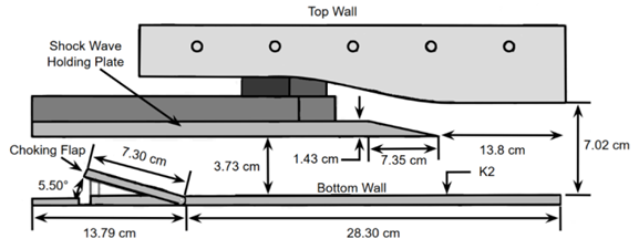Figure 1. Two-dimensional view of test section for experimental measurements. All dimensions are given in centimeters

2.2. Shadowgraph Flow Visualization Apparatus

During wind tunnel tests, a shadowgraph system, described by Manneschmidt and Ligrani [8], records time-varying, shock-wave flow features within the test section. Varying density variations within the flow field are captured using this system within a visualized volume as a line-of-sight integrated image, which covers most of the span of the test section. Time- and spatially-resolved shadowgraph images are captured using an AF Micro NIKKOR 200 mm 1:4D ED camera lens, along with a Phantom v711 high speed camera, which is manufactured by the Ametek Materials Analysis Division of Vision Research Company [7,8].

3. Data Acquisition and Analysis Procedures

Figure 3 shows a flowchart with an overview of data processing procedures.

3.1. Acquisition of Digital Shadowgraph Flow Visualization Data

Phantom Video Player 3.11.11.806 software is employed to process the time sequence video files which are captured using the Phantom camera. The video files are arranged into individual images with a spatial resolution of 20 micrometres per pixel. The exposure time is 1.0 μs and visualization images are acquired at 6.25 kHz. Data processing is accomplished using MATLAB version R2025b software. Additional details are provided by Manneschmidt and Ligrani [8].

3.2. Shock Wave Tracking Determination and Results

Shock wave instantaneous locations are tracked along horizontal pixel group lines that cross the shock wave within each instantaneous visualized digital image. For the configuration with the oblique shock wave with its first reflection, these line placements are solid black and are shown in Figure 2. This figure shows an instantaneous shadowgraph image for one individual digital frame with a variety of oblique shock wave phenomena within the test section. Horizontal lines within this figure show pixel locations within the shadowgraph flow field, along which, shock wave position is tracked upon to determine digitized flow direction locations. The position of the K2 Kulite pressure transducer, used to gather time-varying surface static pressure data, is also included within Figure 2. Manneschmidt and Ligrani [8] describe the analytic procedures employed to determine shock wave position with respect to time, including MATLAB program coding to determine the grey scale pixel intensity across the shock wave for every digitized shadowgraph image.

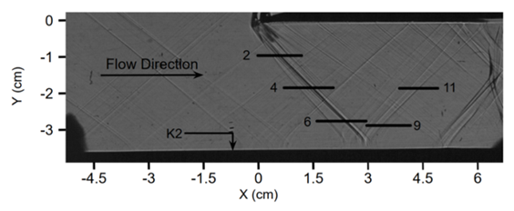Figure 2. Instantaneous shadowgraph image with locations for time lag and magnitude squared coherence analysis along the oblique shock wave and along its first oblique shock wave reflection

3.3. Detailed Data Acquisition and Analysis

The first step in computing distributions of correlation data as they vary with frequency is the application of a 5th order low-pass Butterworth filter that attenuates all frequencies above 90 percent of the Nyquist folding frequency. This is accomplished with the butter function within MATLAB. The application of the mscohere function within MATLAB is then employed to obtain magnitude squared coherence distributions as they vary with frequency. The application of the cpsd function within MATLAB is employed to determine cross power spectral density distributions, which are employed to calculate phase lag and time lag variations as they vary with frequency. Each distribution is determined with a specified number of data segments with 50 percent overlap with adjacent data segments. The data sample length of each segment L_s is calculated using the following equation, where N is the total number of data samples, K is the number of window segments, and D is sample overlap between segments.

(1)

The resulting frequency resolution ΔF is then given by

(2)

where F_s is the data sampling frequency, which, for the present investigation, is set to 6.25 kHz. This approach gives one correlation and time lag distribution for each Hanning window, where one Hanning window is applied to each data segment. The resulting correlation distributions are then ensemble averaged together to provide a single ensemble averaged correlation distribution. The resulting data are valid and presented from ΔF Hz to the Nyquist folding frequency value.

3.4. Magnitude Squared Coherence Determination

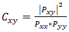
Magnitude squared coherence correlation analysis is used to provide information of flow phenomena which are interacting with each other in a coherent manner at different frequencies. The resulting determined value C_xy quantifies the correlation between two datasets, from 0 to 1, as a function of frequency. With the MATLAB mscohere function, the coherence quantity is expressed using an equation of the form

(3)

where P_xx is the power spectral density of the first signal, P_yy is the power spectral density of the second signal, and P_xy is the cross power spectral density between the two signals. Data produced with the present analysis approach are occasionally very noisy, with greater data scatter as the frequency gets higher. To remedy this issue, 50 points are employed for moving average analysis associated with magnitude squared coherence determinations. The MATLAB function smoothdata with the movmean parameter applied is employed for this purpose. Additional details are provided by Manneschmidt and Ligrani [8].

3.5. Cross Power Spectral Density, Phase Lag, and Time Lag Determination

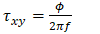
The cross power spectral density P_xy is determined with the cpsd function in MATLAB, and used to calculate the phase lag and the time lag between time sequences of grayscale data associated with two different flow line tracking locations. In regard to cross power spectral density results, the angle of the phase lag is calculated based on the real and imaginary parts of the complex result at each frequency. This is done using the negative of the angle function in MATLAB. Time lag magnitudes are then determined by dividing phase lag ϕ values by associated frequency values, as given by

(4)

Although the phase and time lags are calculated at each discrete frequency between ΔF and the Nyquist folding frequency, the most meaningful phase lag results are at frequencies associated with relatively strong coherence. The time lag is of course a function of frequency. Perturbations occur at a location and propagate to other locations. Time is required for flow perturbations to travel, so the signals detected at two locations are similar, but differ by some time lag. All the perturbations do not originate in the same location, nor do they propagate along the same path at the same rate. Hence, the perturbations at unique frequencies have unique time and phase lags.

Considering the line locations for coherence and time lag analysis shown in Figure 2, determinations of magnitude squared coherence and time lag require the input of data from two separate line flow locations. The sign of the resulting time lag is related to the order of occurrence for the data associated with these locations. With the present arrangement, a negative time lag indicates that the variable which is first inserted into the cpsd function of MATLAB occurs first, and prior to the second inserted variable.

Additional discussion of related details is provided by Manneschmidt et al. [7].

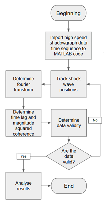Figure 3. Flowchart with overview of data processing procedures

4. Correlation Results which are Unrepresentative of Physical Flow Behavior

4.1. Physically-Unrepresentative Correlation Data Associated with Time Series Data Affected by Transient Wind Tunnel Start-Up Behavior

Within this section, an example of physically-unrepresentative correlation data is provided. The magnitude squared coherence and time lag data shown in Figure 4 are provided for oblique shock wave position 2, relative to oblique shock wave position 6 (Figure 2). Welch’s fast Fourier transform method is employed for analysis. To process the measured experimental results, 31450 frames of data are analyzed with 5 segments for ensemble averaging, with a data overlap for each segment of 50 percent. The resulting segment length and frequency resolution are 10483 and 0.60 Hz, respectively.

The processed time series data includes unsteady motions associated with wind tunnel transient start-up behavior. Associated unsteady contributions are apparent as broad local maximum values within the C_xy data shown in Figure 4, and these are most evident at frequencies of 10 to 50 Hz and 60 to 90 Hz. Establishment of stable flow behavior (without start-up transients) does not occur until after the effects of the start-up transients subside and is not present for a period which is long enough to resolve physically representative unsteady flow events at lower frequencies. The consequence is erroneous and physically unrealistic coherence data, especially for frequencies less than about 100 Hz.

Associated time lag data are thus also generally in error for the same range of frequencies. This is illustrated in Figure 4 by physically unrealistic and inconsistent data for the 2-6 and 6-2 arrangements. These indications are apparent when a reversed sequence of data processing (i.e. 6-2 data) is compared to a forward sequence of data processing (i.e. 2-6 data). Here, a forward sequence of data processing means that data for position 2 are associated with the first correlation input variable, and data for position 6 are associated with the second correlation input variable. A reversed sequence of data processing means that data for position 6 are associated with the first correlation input variable, and data for position 2 are associated with the second correlation input variable.

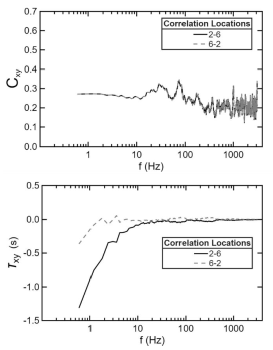Figure 4. Time lag and magnitude squared coherence variations with frequency for oblique shock wave position 2 relative to oblique shock wave position 6

Inconsistency and errors within the forward 2-6 and reversed 6-2 data sets in Figure 4 are present. The physically unrealistic character of these time lag data within Figure 4 is indicated by 2-6 and 6-2 data sets which are not symmetrical relative to a zero value of time lag, resulting in contradictory information regarding the sequence of data set occurrence. In contrast, correct and physically-representative time lag measurements are characterized by two quantitatively similar distributions, with opposite signs at each frequency, and symmetric variations with respect to each other, relative to a time lag value of zero. The resulting two sets then give physically-representative behavior with similar indications regarding which data set occurs first and which data set occurs second.

4.2. Physically-Unrepresentative Correlation Data Associated with Too Many Segments for Ensemble Averaging

Here, a second example of physically-unrepresentative correlation data is provided. The magnitude squared coherence and time lag data shown in Figure 5 are obtained from measured samples with 31450 frames of data. To obtain the results shown in this figure, 15 segments are employed for ensemble averaging, and the data overlap employed for each segment is 50 percent. The resulting frequency resolution and segment length are 1.60 Hz and 3971, respectively. Results shown in Figure 5 are obtained for oblique shock wave position 2, relative to position 9, which is associated with the first oblique reflection of the oblique shock wave.

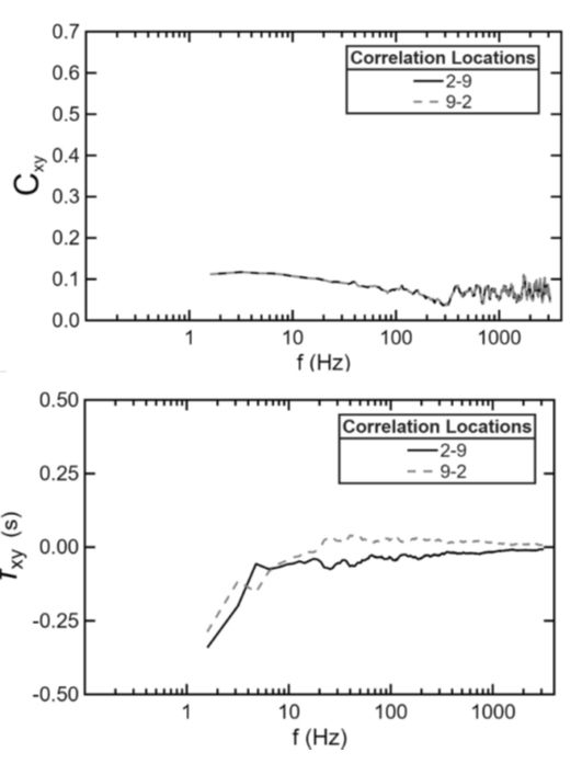Figure 5. Time lag and magnitude squared coherence variations with frequency for oblique shock wave position 2 relative to oblique shock wave reflection position 9

The τ_xy and C_xy data within Figure 5 with 15 segments show minimal scatter at higher frequencies greater than 500 Hz. Such characteristics are partially a consequence of the use of larger numbers of segments, which generally result in smoother distributions, with lower variance. Reduced frequency resolution is also a consequence of the data processing arrangement which is employed. The resulting C_xy magnitude squared coherence distribution is incorrectly low for most all frequencies considered, with magnitudes aligned with background noise levels. As a result, no significant correlation events are evidenced by the C_xy data within Figure 5. Note that this lack of correlation is also a partial consequence of the relatively poor resolution and lack of contrast associated with the reflected oblique shock wave as its unsteady characteristics are captured at position 9.

The time lag distributions presented within Figure 5 also show anomalous characteristics. These data are presented as signals associated with positions 2 and 9 are analyzed with both forward and reverse insertion into the time lag software. Results from this code are provided such that a negative time lag means that the first inserted signal occurs first, and prior to the second signal. The data within Figure 5 thus indicate that events at position 2 occur first within the 2-9 data set, and that events at position 9 occur first within the 9-2 data set. The absolute values of the time lag values within the distributions which demonstrate these characteristics are also excessively and unrealistically large, especially for frequencies less than 10 Hz. Such characteristics are partially a consequence of reduced frequency resolution, indicating that results in Figure 5 (obtained with 15 segments employed for ensemble averaging) are generally in error and unrepresentative of actual oblique shock wave flow behavior, especially when the associated C_xy data are also considered.

4.3. Physically-Unrepresentative Correlation Data Associated with Too Few Segments for Ensemble Averaging

Magnitude squared coherence and time lag data obtained with too few segments for ensemble averaging are also not representative of true physical behavior. Too few segments also result in longer segment lengths, and data distributions which are less smooth, with greater noise, higher variance, and increased frequency resolution. For example, if 3 segments are employed with 31450 frames of data, and data overlap for each segment of 50 percent, the resulting C_xy magnitude squared distribution shows significantly greater scatter at frequencies greater than 300 Hz (relative to high frequency data shown in Figure 5). In addition, C_xy variations show physically unrealistic trends, especially as frequency increases further beyond 100 Hz. Time lag distributions are also largely physically unrealistic, indicated by absolute values which are often unrealistically and excessively large.

4.4. Physically-Unrepresentative Correlation Data Associated with Too Few Time Series Data Points

Physically incorrect magnitude squared coherence and time lag data also result when insufficient data frames are employed for analysis of correlation quantities. With this situation, the period for the acquisition sequence is not long enough for local unsteady behavior to be well established, and insufficient to resolve unsteady events at lower frequencies. This means that time-varying events occurring at the lowest frequencies are largely unresolved and not completely included for correlation parameter determination. Too few datapoints for analysis also cause the correlation analysis algorithms to be unable to distinguish true physical relationships from random signal variations. As a result, coherence data often does not evidence any significant correlation events, indicated by minimal magnitude variations with frequency, and magnitudes that are in the vicinity of background noise levels. Time lag data then often show minimal variations with frequency, without any signatures which evidence significant correlations between flow events at different spatial locations.

4.5. Physically-Unrepresentative Correlation Data Associated with Data Which are Not Well Defined and Too Distant

Erroneous correlation data also result when analysis is applied to two physical locations which are separated from each other by a relatively large distance, or when gray scale data are not well defined, with insufficient contrast between the phenomena of interest and surrounding spatial regions. Within the present investigation, such visualization contrast defects are further exacerbated by unsteady transient motions of the recorded flow phenomena. The consequence is that the correlation algorithm does not accurately track unsteady phenomenological motions. In addition, phase shift values are dominated by noise, and are thus, in error for most considered frequency values. The result is contradictory and physically incorrect time lag and magnitude squared coherence information, with coherence values that are often not discernable, relative to background noise.

5. Correlation Results Which are Representative of Physical Flow Behavior

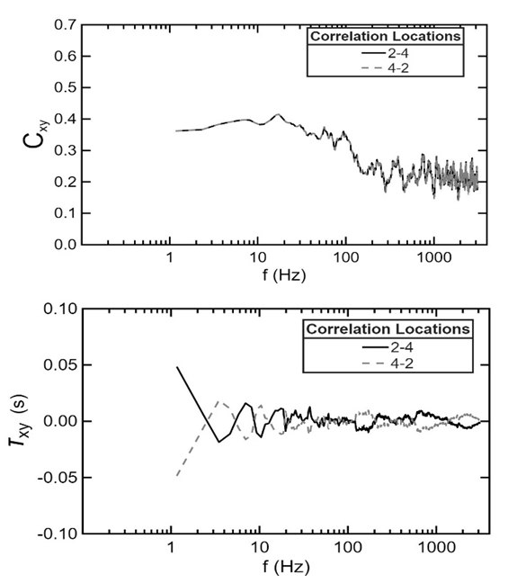
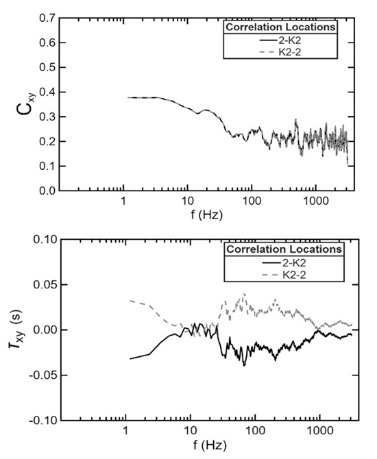
Figures 6 and 7 present physically-representative correlation data. The time lag and magnitude squared coherence variations with frequency results shown in Figure 7 are associated with oblique shock wave position 2 relative to oblique shock wave position 4. The time lag and magnitude squared coherence variations with frequency results shown in Figure 6 are associated with oblique shock wave position 2 relative to Kulite transducer K2. Shock wave positions 2 and 4 and the location of the K2 Kulite pressure transducer are shown in Figure 2, which presents an instantaneous shadowgraph image with identified line locations (relative to the oblique shock wave and its first reflection) for time lag and magnitude squared coherence analysis.

Figure 6. Time lag and magnitude squared coherence variations with frequency for oblique shock wave position 2 relative to Kulite transducer K2

Figure 7. Time lag and magnitude squared coherence variations with frequency for oblique shock wave position 2 relative to oblique shock wave position 4

The data shown within Figures 6 and 7 are obtained with Welch’s approach for fast Fourier transform analysis, and 5 segments of data for ensemble averaging, where the overlap for each segment is 50 percent. The number of frames of data employed for analysis is 16150. The resulting frequency resolution is 0.86 Hz. Here, an overlap value of 50 percent helps mitigate the loss of information at the segment edges caused by the windowing function. The use of 5 segments is the optimal value to obtain physically representative data, as determined in relation to the data processing errors which are present when too few or too many segments are employed.

The associated data are acquired and processed to avoid effects leading to physically incorrect results. For example, the beginning of data acquisition occurs after wind tunnel start-up transients are present, and the end of data acquisition occurs before wind tunnel shut-down transients are present. The time interval for data acquisition is 2.58 seconds, which is long enough for adequate resolution of data at lower frequencies. Acquisition sampling frequency is 6.25 kHz, which is large enough to capture high frequency content up to about 3.0 kHz. This acquisition rate, the overall time interval for data acquisition, the use of Welch’s approach, and the use of 5 segments for ensemble averaging then give frequency resolution values which are appropriate for the flow environment. According to the shadowgraph image in Figure 2, locations for flow analysis are in reasonable proximity to each other. Each local shock wave signature is also reasonably well defined with relatively sufficient contrast within grey-scale images for each line sampling location. Resulting unsteady signals within shadowgraph time sequences are then also reasonably well defined as time-varying data are acquired for Fourier correlation analysis.

With these arrangements in place, resulting data in Figures 6 and 7 are correctly representative of physical flow phenomena associated with different flow locations relative to the oblique shock wave. For example, magnitude squared coherence data within Figure 7 show values as high as 0.42, with values generally ranging above 0.37, at frequencies less than around 30 Hz. Such behaviour evidences fluid motions which are strongly correlated between oblique shock wave at position 2 and the oblique shock wave position 4. Also evident within this figure is a relatively smooth C_xy distribution as frequency varies, especially for frequencies less than about 150 Hz. As such, no extra local maxima or peaks are evident, especially for lower frequencies, which indicate that large-scale transient behaviour associated with wind tunnel start-up and shut-down transients is not present. The coherence data in Figure 6 for Kulite transducer K2 and oblique shock wave position 2 evidence a similar conclusion. This is also because of a smooth C_xy distribution as frequency varies at frequencies less than about 100 Hz. Here, substantial magnitude squared coherence values associated with the two signals are generally present, with C_xy as high as 0.38 as frequency decreases to 0.86 Hz.

Time lag values in Figure 7 are generally very small, with absolute values always less than 0.05 seconds for all considered frequencies. This means that oblique shock wave positions 2 and 4 events are almost simultaneous, which is consistent with the strong correlation of flow phenomena associated with these two types of events, especially at lower frequencies (discussed previously). These characteristics are also consistent with the close spatial proximity of positions 2 and 4. Time lag data traces within Figure 7 are included for the forward and reverse insertion of signals from positions 2 and 4 (such that data are provided both with the position 2 signal inserted first, and with the position 4 signal inserted first). Physically correct behaviour of the time lag distribution is evidenced by the resulting two sets of data, because they are mirror images of each other, with asymmetric pattern relative to the zero time lag value. Resulting data within Figure 7 show time lag magnitude and sign alterations as frequency varies, which, depending upon the frequency, indicate either that events associated with position 2 occur first, or that events associated with position 4 occur first. This alteration of event propagation direction with frequency is generally present within Figure 7 for all considered frequencies.

Figure 6 shows similar quantitative trends of time lag magnitudes in regard to correlation of oblique shock wave position 2 events and Kulite K2 sensor signals, since absolute values are always less than 0.04 seconds for all considered frequencies. Here, as for the previous data, reversing the order of data insertion gives two sets of data which are mirror images of each other, with a symmetric pattern relative to the zero time lag value. Figure 6 time lag absolute values are slightly higher (relative to values at other frequencies), in the vicinity of 0.03 seconds at frequencies less than 3 Hz and for frequencies between 25 Hz and 500 Hz. Within these frequency intervals, evidence is provided that oblique shock wave position 2 events are occurring prior to K2 Kulite sensor events, with a time delay between events in the vicinity of 0.03 seconds.

6. Summary and Conclusions

Provided is direction, based upon laboratory data and analysis, in applying existing analytic techniques for coherence analysis to complex time-varying, three-dimensional physical environments. To accomplish this goal, and to avoid the production of incorrect, erroneous data, a variety of measurement scenarios are described (with both positive and negative outcomes) using measurements from an application environment containing compressible, shock wave phenomena. Visualized image data from such shock wave flow environments are well suited for the development of appropriate methodologies for coherence determination because of the complexity of the time-varying flow fields, and because of the challenges in obtaining physically representative coherence data.

The present investigation considers magnitude squared coherence and time lag determination within a compressible shock wave flow environment with an oblique shock wave with its first reflection. Laboratory configuration and analysis details are provided for determination of these quantities, which lead to physically-representative correlation data. Because extra challenges are present for correlation determinations, laboratory configuration and analysis arrangements are also considered and provided, which lead to physically-unrepresentative data, generally with extensive errors. The results from the present study (including acquisition and analysis procedures used to obtain these results) are broadly applicable to any environment which requires correlation of events which are changing with time in a broad band manner, as they are separated by different physical locations. Such application environments include ones which are associated with neurosciences, civil engineering, geological phenomena, seismology, structural mechanics, as well as a variety of other academic disciplines.

Flow arrangements which are employed to give physically-unrepresentative results include transient wind tunnel start-up events which are present as time series data are acquired, and the employment of flow locations (which are utilized for data analysis) which are too far distant from each other. The use of time-varying data, which are not well defined or are present without sufficient contrast, is also found to lead to physically-unrepresentative results. Data analysis and acquisition arrangements which lead to similar issues include the use of a multitaper approach for fast Fourier transform analysis, the use of too few time series data points, the use of too many segments for ensemble averaging, and the use of too few segments for ensemble averaging. Note that changing the last three of these parameters leads to alterations of data segment sample length and frequency resolution. Time lag variations with frequency are a sensitive indicator of physically-unrepresentative data. Indications of such behaviour are provided by forward and reversed sequence data processing arrangements which give time lag versus frequency distributions, which are not symmetric with respect to each other, relative to a zero value of time lag. Such symmetry is an important detector of unrepresentative data because symmetric data for both forward and reversed data processing sequences means that both resulting time lag data sets give the same conclusion regarding the time sequence of data occurrence. In contrast, magnitude squared coherence variations with frequency generally change by imperceptible amounts as data associated with forward and reversed data sequence arrangements are compared, even though parameters or conditions associated with unrepresentative behaviour are present.

With these considerations in mind, physically-representative correlation data are obtained for an oblique shock wave arrangement with Welch’s approach for fast Fourier transform analysis. The frequency resolution for the data is 0.86 Hz, with 5 segments of data employed for ensemble averaging, where the overlap for each segment is 50 percent. To avoid the acquisition and processing of physically incorrect data, the beginning of data acquisition occurs after wind tunnel start-up transients are present, and the end of data acquisition occurs before wind tunnel shut-down transients are present. The time interval for oblique shock wave data acquisition is 2.58 seconds, which is long enough for adequate resolution of data at lower frequencies. Acquisition sampling frequency is 6.25 kHz, which is large enough to capture high frequency content up to about 3.0 kHz. This acquisition rate, the overall time interval for data acquisition, the use of Welch’s approach, and the use of 5 segments for ensemble averaging then gives a frequency resolution value which is appropriate for the flow environment. In addition, locations for flow analysis are in reasonable proximity to each other, with local shock wave shadowgraph signatures which are reasonably well defined with relatively sufficient contrast within grey-scale images for each line sampling location. Resulting unsteady signals within shadowgraph time sequences are then also reasonably well defined as time-varying data are acquired for Fourier correlation analysis.

ACKNOWLEDGEMENTS

The present research effort was funded by the CBET Thermal Transport Processes Program, National Science Foundation, Award Number 2041618.