1. Introduction

The quantity of data available for statistical analysis is growing at an increasingly faster rate. This phenomenon requires new and better probability distributions to handle such datasets in real-life situations. Given this requirement, several generalised distributions have been proposed in the literature by researchers. The importance of these new distributions is paramount because no single distribution can fit all situations; hence, continual research to propose new distributions. Some of the proposed families of distributions in literature include: exponentiated generalised class of distributions [1], beta generalised class of distributions [2], MacDonald generalised class [3], Kumaraswamy generalised class of distributions [4], Marshall-Olkin class of distributions [5], and Gamma generated class of distributions [6], among others. Many of these developed families of distributions are algebraic, and recently, attention is shifting towards the development of statistical distributions based on trigonometric functions. This new paradigm has diverse potential for researchers to explore. It offers researchers many alternatives regarding the availability and suitability of distributions. Some examples of trigonometric function-based distributions include secant generated class of distributions [7], the sine Kumaraswamy-generated class of distributions [8], cosine cosine-generated class of distributions [9], new extended cosine generalised class of distributions [10], cotangent trigonometric-G class of distributions [11], Tangent generalised class of distributions [12] and recently, secant Kumaraswamy Class of distributions [13] among others. The article chose the cosine function over the sine function due to the following reasons. The cosine-based forms are easier to use directly as probability densities. Cosine is an even function that has a natural symmetric probability distribution as compared to sine, which is an odd function, making it less straightforward as a generator. Cosine functions often have closed forms as compared to sine functions. Cosine-based probability distribution functions are important in modelling bounded lifetimes with symmetric failure rates. It can represent bathtub-shaped or periodic hazard rates and approximate survival functions using Fourier cosine expansions, which include real-world failure patterns in systems under cyclic or periodic stress in reliability studies.

Other sections of the article are presented as follows: section 2 covers the development of the proposed cosine Kumaraswamy class of distributions, section 3 covers the mixture form of the density, statistical properties are discussed in 4, parameter estimations are covered in Section 5, special cases of the proposed class are presented in section 6, whilst section 7 deals with Monte Carlo simulation. Not only are applications to lifetime data presented in Section 8, but the log-location-scale regression model is covered in Section 9. Finally, a summary of the paper is presented in Section 10.

2. Cosine Kumaraswamy Class of Distributions

The cosine generalised (cosine-G) class of distributions [9] is established to be more flexible and efficient in fitting many lifetime data in survival and reliability modelling. The cumulative density function (CDF) of the Cosine-G is given as,

where is the parent distribution. Also, the CDF of the Kumaraswamy generated (KG) class of distributions [4] is given as,

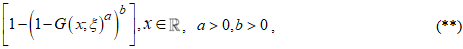
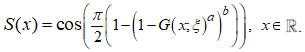
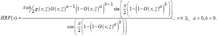
where is the baseline distribution. Substituting equation (**) into equation (*) yields the CDF of the new class of distribution known as the Cosine Kumaraswamy generalised (CKG) class of distributions, denoted by F(x), which is presented as

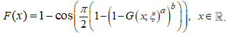(1)

The survival function of the CKG class of distributions is defined as the probability that a patient, or a device, will survive beyond a certain time, and it is obtained by subtracting the CDF from one. This is given as

(2)

The probability density function, f(x), of the CKG is obtained by differentiating equation (1), and it is given as

(3)

The hazard rate function (HRF) measures the instantaneous risk of an event, such as failure or death, occurring at a specific time given that it has not happened before that time. It is obtained as the ratio of the PDF to the survival function, and it is presented as

(4)

3. Mixture Representation of CKG Class

This section focuses on the mixture representation of the PDF of the CKG distribution. The mixture representation is very useful when deriving the statistical properties of the CKG distribution.

Lamma 1. The mixture representation of the CKG distribution is obtained as

,

Where

Proof. Given the PDF of the CKG distribution

Using the Binomial series expansion of gives

.

Using the expanded form of the term involving the sine function as defined by [10], yields

.

The mixture form of the PDF is finally presented as

(5)

Where

4. Statistical Properties

The statistical properties of the CKG class of distributions are derived in this section. The properties considered are the quantile, moments, moment-generating function, incomplete moments, order statistics, and mean residual life.

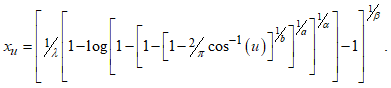
4.1. Quantile Function

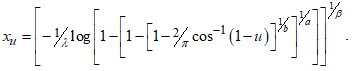
A quantile function is essential for the generation of random numbers of a given distribution. The quantile function of the CKG class of distribution for is given as

(6)

where denotes the quantile function of the baseline model.

Proof. Equating equation (1) to , and expressing in terms of the other variables. The quantile function of the CKG class of distribution is presented as;

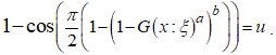Re-arranging gives

Taking the inverse of the cosine function of both sides gives

The expression for is obtained as

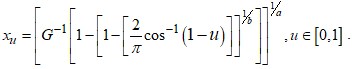
4.2. Moments

Moments are essential in determining measures of central tendency, dispersion, and variation of data.

Proposition 2: The non-central moment of the CKG class of distributions is defined by

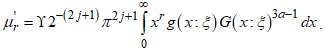(7)

Proof: The non-central moment is defined as,

Substituting equation (5) in place of the term yields

4.3. Incomplete Moments

The incomplete moment is essential in calculating the mean deviation and measures of inequality, such as Bonferroni curves and Lorenz curves.

Proposition 3: The incomplete moment of the CKG is defined as

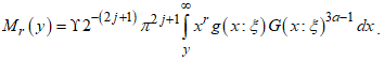(8)

Proof. The incomplete moment of is defined as follows:

After substituting the mixture form into the definition, the incomplete moment is

4.4. Moment-Generating Function

Proposition 4. If for any integer value, the moment-generating function is

(9)

Proof. The moment-generating function is defined as follows;

Using the Taylor series:

Implies,

But as obtained in equation (), then

4.5. Order Statistics

Order statistics are prevalent variables used for modelling some lifetime systems in various component structures. The focus of this subsection is to derive the order statistics of the CKG distribution.

Proposition 5: The order statistic of the random sample of the CKG is presented as

(10)

Proof. The order statistic of the random sample is the random variable , where

is the ordered sample. Accordingly, the PDF of is,

Using the Binomial series expansion for the term,

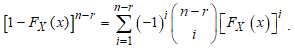Then, substituting the new term for into equation (10) gives,

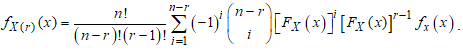This is simplified as,

Substituting the PDF in equation (2) and CDF in equation (2) gives the order statistics as

where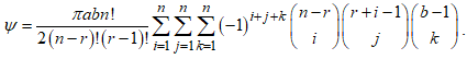

4.6. Inequality Measures

The Lorenz and Bonferroni curves are the primary methods for measuring income inequality. It is also applicable in measuring the inequality in the survival times of patients suffering from cancer and other related conditions.

Proposition 6: If , then the Lorenz curve is defined as:

(11)

Proof: The Lorenz curve is defined as:

where is the first incomplete moment given in equation (8).

Hence, substituting equation (8) into the Lorenz curve function gives:

4.7. Mean residual life

In life testing situations, the mean residual life function is defined as the expected additional lifetime given that a component has survived until time t. It is the average time that units in the population are expected to operate before failure. It is very useful in both reliability and survival analysis.

Proposition 7: If has the CKG distribution, then the mean residual life function, is defined as:

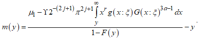(12)

Proof. The mean residual life function, is defined as:

It is expressed as;

and further expressed as;

5. Parameter Estimation

This section discusses the maximum likelihood estimation and the ordinary least squares methods of parameter estimation. These methods are used to obtain the estimates of the parameters of the CKG distribution.

5.1. Maximum Likelihood

Let be a random sample from a population with PDF , where the parameter is not known. If is the likelihood function of the distribution, then

The value that maximizes is called the maximum likelihood estimator of and is denoted by or just by and is called the maximum likelihood estimate of . The maximum likelihood estimate is . The method of maximum likelihood, in a sense, picks out of all the possible values of the most likely to have produced the given observations . The likelihood of the CKG class of models is given as

(13)

The log-likelihood equation is given as

(14)

Taking the partial derivative of equation (14) with respect to the parameters yields the following

(15)

and

(16)

5.2. Ordinary Least Squares Estimation Method

The ordinary least squares (OLS) estimation method minimises the objective function. If are the order statistics of a random sample of size obtained from the CKG model. The OLS estimates and for the CKG class of distributions, parameters can be obtained by minimising the objective function,

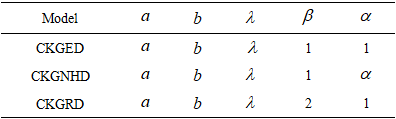
6. Special Cases of the CKG Class

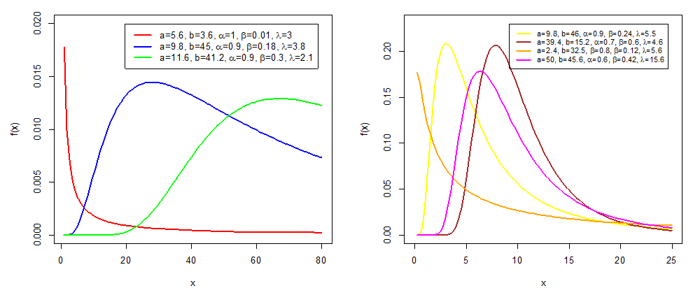
In this section, we discuss the generalisations of some distributions using the CKG class of distributions. The first model considered is the cosine Kumaraswamy Weibull (CKW) distribution. The study investigates the characteristics exhibited by its PDF as well as its hazard failure rates.

6.1. Cosine Kumaraswamy Weibull Distribution

Using the Weibull distribution [14] as the baseline distribution, its CDF and PDF are given as and , respectively.

The CDF of the CKW is obtained by substituting into equation (1). This is obtained as

(17)

Differentiating equation (17) gives the PDF of the CKW distribution and is presented as

(18)

Figure 1 shows the various shapes exhibited by the PDF of the CKW distribution. Some of the shapes include increasing and decreasing. Others are negatively and positively skewed with different kurtosis.

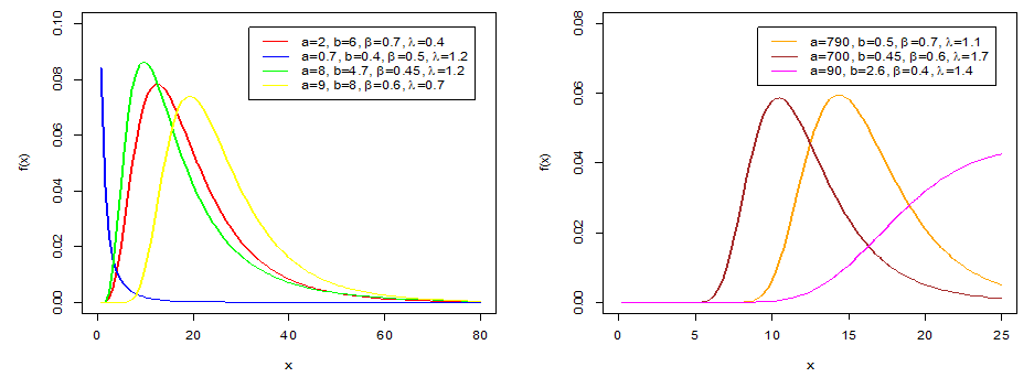Figure 1. CKW PDF shapes

The hazard function of the CKW distribution is obtained by dividing the PDF function by the survival function. This gives

(19)

The hazard failure rate shows bathtub, unimodal, increasing, and decreasing shapes. The details are shown in Figure 2.

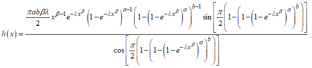
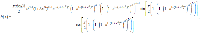
Figure 2. CKW hazard function shapes

The CKW model has a quantile function presented as

(20)

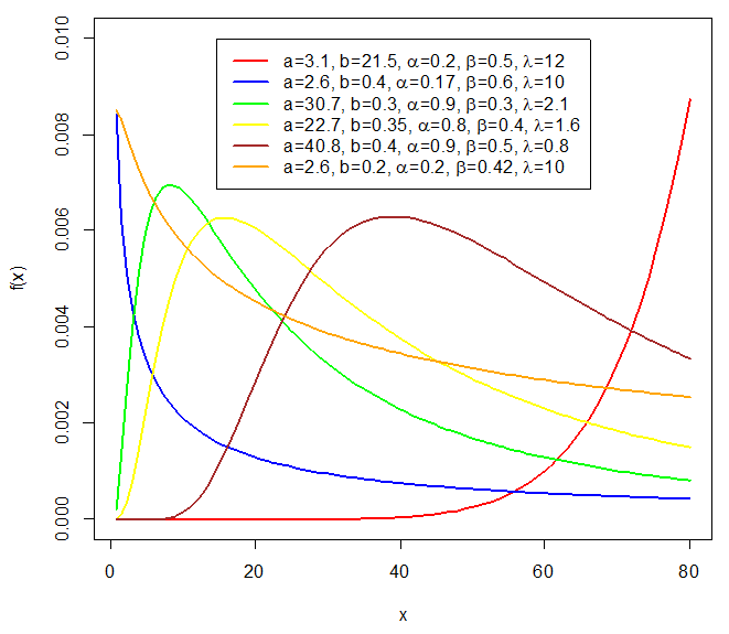
6.2. Cosine Kumaraswamy Generalised Power Weibull

The second model derived from the CKG distribution is the Cosine Kumaraswamy's generalised power Weibull (CKGPW) distribution. Suppose the baseline distribution is the generalised power Weibull distribution as defined by [15]. The CDF and PDF of the CKGPW are presented as and respectively, where and .

The CDF of the CKGPW is obtained by substituting into equation (1) and is presented as

(21)

Differentiating equation (21) gives the PDF of the CKGPW, which is presented as

(22)

The desirable shapes that characterise its PDF include positively skewed, decreasing, reversed-J, and increasing shapes. The details are shown in Figure 3.

Figure 3. CKGPW PDF shapes

The CKGPW has its hazard function presented as the ratio of its PDF to its survival function. This is presented as

(23)

The desirable shapes associated with the failure rate of the CKGPW are upside-down bathtubs, increasing and decreasing as shown in Figure 4.

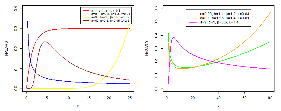
Figure 4. Failure rate of the CKGPW

The CKGPW distribution converges to other important distributions with certain values of its parameters. If the following sub-models are obtained for some parameter values.

1. For and the PDF becomes the cosine Kumaraswamy exponential distribution (CKGED).

2. For , the PDF assumes into the cosine Kumaraswamy generalised Nadarajah-Haghighi distribution (CKGNHD).

3. When and the PDF assumes the cosine Kumaraswamy generalised Rayleigh distribution (CKGRD), which is also a new model.

This is summarised in Table 1.

Table 1. Sub-models of the CKGPWD

The quantile function of the CKGPW is presented as

(24)

7. Simulation

To examine how the parameters behave under maximum likelihood and ordinary least squares estimators, Monte Carlo simulations are carried out using the CKW model. The following procedures were undertaken in the simulation process:

a. Create random samples with sizes 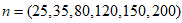using the quantile function of the CKW model.

b. Using least squares and maximum likelihood, estimate the parameters by calculating the average bias (AB) and root mean square error (RMSE) expressed as follows:

c. The procedure is replicated 1000 times.

d. This procedure is done for both MLE and OLS methods of parameter estimation .

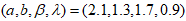The results of the simulation process are shown in Table 2. The results show that the estimators are unbiased and consistent as the AB and RMSE estimates approach the true values, and the estimates decrease with increasing sample sizes. The rate of convergence in the maximum likelihood estimator is faster than the ordinary least squares estimator.

Table 2. Simulation results for the CKW parameters

8. Applications

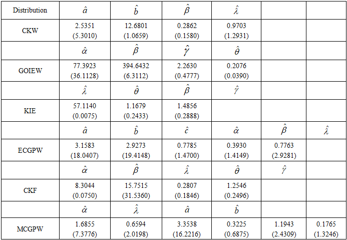
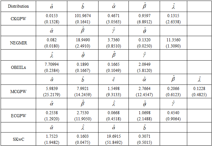
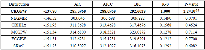
In this section, the flexibility of the special cases of the CKG class of distributions is examined. The CKW and CKGPW distributions are compared with some existing models such as new generalised modified odd inverse exponential Weibull (GOIEW) [16], Kumaraswamy inverse exponential (KIE) [17], extended cosine generalised power Weibull (ECGPW) [18], MacDonald generalised power Weibull (MCGPW) [19], exponential Lomax (ELx), [20], secant Kumaraswamy Weibull (SKW) [13], odd-Burr III Lomax [21] (OBIIILx) and generalised modified inverse Rayleigh (GMIR) [22].

8.1. First Dataset

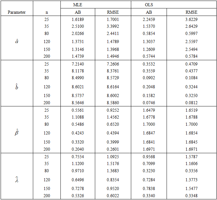
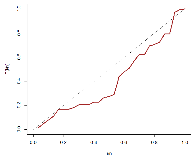
The first dataset represents the survival times of patients suffering from head and neck cancer. The patients were treated with a combination of radiotherapy and chemotherapy (RT and CT). The dataset can be found in [23].

12.20, 47.38, 81.43, 127.00, 173.00, 319.00, 817.00, 23.56, 55.46, 84.00, 130.00, 179.00, 339.00, 1776.00, 23.74, 58.36, 92.00, 133.00, 194.00, 432.00, 25.87, 63.47, 94.00, 140.00, 195.00, 469.00, 31.98, 68.46, 110.00, 146.00, 209.00, 519.00, 37.00, 78.26, 112.00, 155.00, 249.00, 633.00, 41.35, 74.47, 119.00, 159.00, 281.00, 725.00.

The descriptive statistics of the cancer dataset show a mean value of 223.5 and a median value of 128.5. Since the mean is greater than the median, it indicates that the data is highly skewed to the right with a skewness value of 3.50. The dataset also reports a standard deviation of 305.4, leptokurtic (higher than the normal distribution), and with a kurtosis value of 15.3. The summary is presented in Table 3.

Table 3. Descriptive statistics for the first dataset

The total time on test (TTT) transform graph of the head-neck dataset is presented in Figure 5. It indicates that the failure rate of the dataset has a bathtub shape. This is because the curve moves initially from above the diagonal and then goes below it.

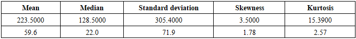
Figure 5. TTT graph of the first dataset

The MLE of the parameters of the CKW and other existing distributions are shown in Table 4. The corresponding standard errors are shown in parentheses.

Table 4. Parameter estimates of the first dataset

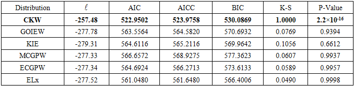
The performance of the CKW and other fitted distributions is compared using Akaike information criteria (AIC), corrected Akaike information criteria (AICc), Bayesian information criteria (BIC), log-likelihood (), and Kolmogorov-Smirnov (K-S). The underpinning statement for comparison is that a model with the highest value of log-likelihood, K-S and the smallest values of AIC, AICc, and BIC has better performance in fitting the given dataset.

The goodness-of-fit statistics of the fitted distributions have been examined, and the results are presented in Table 5. The proposed model in bold has better fitted the head and neck dataset than the other competing models, as indicated by the criteria statement above.

Table 5. Goodness-of-fit measures for the first dataset

The variance-covariance matrix for the head-neck dataset is obtained and presented as follows

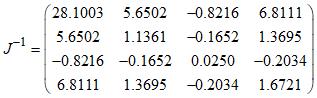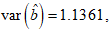
The variances of the MLE of the parameters for the CKW distribution with the head-neck dataset are: . and . The ninety-five per cent (95%) confidence intervals of the estimated parameters are respectively obtained as (0, 12.9251), (10.5909, 14.7693), (0, 0.5959), and (0, 3.5048).

The empirical PDF and CDF plots of the competing models are shown in Figure 6. The proposed CKW models have mimicked the empirical plots better than the other competing models.

Figure 6. Models’ PDF and CDF plots for the first dataset

The P-P plots of the competing models for the head-neck dataset are examined and presented in Figure 7. The CKW model has the majority of its plotted points on the diagonal line, compared to the other models.

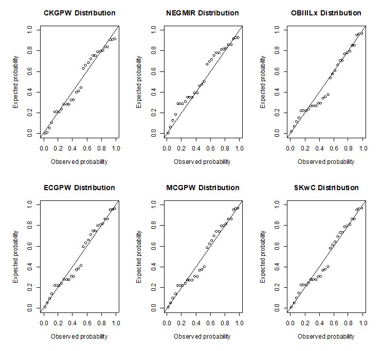
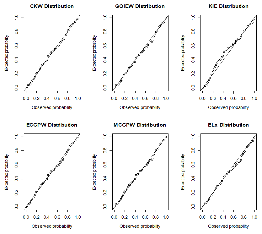Figure 7. Models’ P-P plot for the first dataset

8.2. Second Dataset

The second dataset comprises a random sample of 30 observations of the failure times of an aircraft air conditioning system. The dataset can be found in [24].

23, 261, 87, 7, 120, 14, 62, 47, 225, 71, 246, 21, 42, 20, 5, 12, 120, 11, 3, 14, 71, 11, 1, 4, 11, 16, 90, 1, 16, 52, 95.

The descriptive statistics of the aircraft dataset show a mean value of 59.6 and a median value of 22.0. The dataset is positively skewed with a skewness value of 1.78. The dataset also reports a standard deviation of 71.9 and is more moderately peaked than the normal distribution, with a kurtosis value of 2.57 as shown in Table 6.

Table 6. Descriptive Statistics for the second dataset

The TTT transform plot for the aircraft dataset is presented in Figure 8. The plot shows a bathtub failure rate.

Figure 8. TTT transform plot for the second dataset

The MLE of the parameters of the CKGPW and other existing distributions are shown in Table 7. The corresponding standard errors are shown in parentheses.

Table 7. Parameter estimates for the second dataset

The goodness-of-fit statistics results are presented in Table 8 for the aircraft dataset with the proposed model in bold.

Table 8. Goodness-of-fit measures for the second dataset

The variance-covariance matrix of the CKGPW distribution for the aircraft dataset is obtained as

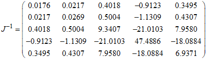The variances of the MLE of the parameters for the CKW distribution with the head-neck dataset are , and 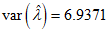. The ninety-five per cent (95%) confidence intervals of the estimated parameters are respectively obtained as: (0, 0.0588), (101.6458, 102.2890), (0, 6.4575), (0, 14.4665), and (0, 5.2938).

The empirical PDF and CDF plots with the competing distributions are presented in Figure 9.

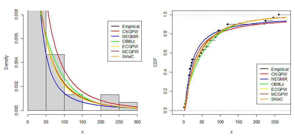Figure 9. Models’ PDF and CDF plots for the second dataset

The P-P plots of the competing models for the aircraft dataset are examined and presented in Figure 10. The CKGPW model has its plotted points on the diagonal better than the other distributions.

Figure 10. Models' P-P plots for the second dataset

9. Location-scale Regression Model

In this section, a regression model is developed for the CKW distribution. The model developed is known as the log location-scale cosine Kumaraswamy regression model and is denoted by (LCKW). It is obtained by the transformation of the random variable and the following re-parametrization are applied, and . Using equation (17), the CDF of the CKW model is denoted as . Also given that and . Then the CDF of the LCKW regression model is obtained as

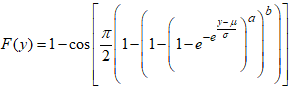(25)

Where

The LCKW regression has a survival rate function as

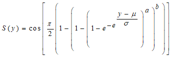(26)

Consequently, the PDF of LCKW can be obtained by differentiating equation (25) and is presented as

(27)

Where

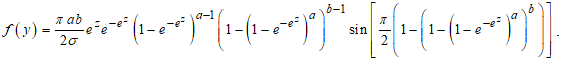
The LCKW regression model is of the form:

where is the location parameter, is the vector of covariates, is the vector of regression coefficients and the is the error term. The parameters of the regression model are estimated using equation (27) with the aid of the maximum likelihood estimation method. The log-likelihood function is given as

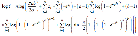(28)

The estimates of the parameters are obtained by maximising the log-likelihood function in equation (28). The adequacy of the LCKW location-scale regression model is examined using the Cox-Snell residuals [25].

The Cox-Snell residuals of the LCKW location-scale regression model are , where is defined in equation (29). If the LCKW location-scale regression model fits the given data well, its Cox-Snell residuals are expected to follow the standard exponential distribution.

9.1. Third Dataset

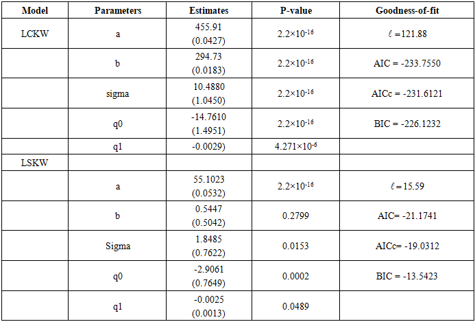
The dataset contains values for long-term interest (LTI) and foreign direct investment (FDI), available in [26]. The usefulness of the LCKW regression model is highlighted using this dataset.

LTI rate (%): 2.640, 0.596, 0.680, 2.190, 4.560, 2.140, 0.410, 0.530, 0.750, 0.280, 4.390, 3.390, 5.190, 0.800, 2.160, 2.640, 0.060, 2.549, 0.930, 0.310, 0.540, 7,750, 0.470, 2.810, 1.760, 3.170, 1.760, 1.010, 0.990, 1.318, 0.550, 0.040, 1.374, 2.890.

FDI stocks outward (% GDP): 30.78, 57.87, 121.52, 90.17, 45.39, 11.08, 55.92, 51.54, 56.31, 43.34, 11.64, 20.85, 21.99, 276.22, 28.81, 27.56, 30.60, 21.02, 5.93, 7.24, 380.10, 15.76, 305.44, 8.94, 48.05, 5.41, 23.68, 3.56, 14.53, 41.90, 71.70, 162.75, 61.86, 40.43.

The performance of the LCKW location-scale regression model is compared with some existing regression models in the literature, such as the log secant Kumaraswamy Weibull location-scale regression model [13]. The parameter estimates for the regression model are obtained using the mle2 function in the bbmle package for R. The computational challenges of the mle2 function usage include evaluation failure, especially if the starting values cause negative scale, zero division or logarithm of zero, mle2 gives out an error and slow convergence is experienced with high-dimensional models if the initial guess is poor and the Hessian may be ill-conditioned at convergence, giving unreliable standard error estimates The MLE estimates and their respective standard errors which are brackets, as well as goodness of fit statistics, are presented in Table 9. The estimates presented in Table 9 show that all the parameters estimated in the LCKW regression are significant. Both the slope and the coefficient of the FDI in the LCKW regression model are negative, which suggests that a unit change in the FDI decreases the LTI rate. From Table 9, the LCKW regression model is presented as: The suitability of the LCKW model is examined with the aid of the Cox-Snell residual as indicated above.

Table 9. Location-scale regression parameter estimates

The P-P plots for the two models are presented in Figure 11. The P-P plot of the LCKW seems to have more of its plots on the diagonal, as the goodness-of-fit statistics indicated.

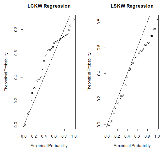Figure 11. P-P plot for the investment dataset

10. Conclusions

The cosine Kumaraswamy class of distributions was developed and studied. The study captures certain statistical features, which include the moment generating function, moments, and quantile function. The others are order statistics, incomplete moments, and measures of inequalities. The study showcased the flexibility of the class of models with three illustrative examples using Weibull, Generalised power Weibull, and new Weibull Pareto distributions. Maximum likelihood and ordinary least squares estimation methods were used to obtain the estimates of the parameters, and a Monte Carlo simulation was undertaken to demonstrate the consistency and robustness of the estimators. The maximum likelihood estimation method performed better than the ordinary least squares method. In addition, the cosine Kumaraswamy model was used to develop a location-scale regression model. Three different lifetime datasets were employed to showcase the applicability, versatility, and efficiency of the proposed models. The outcome indicated that the proposed models have performed better than the existing models. Hence, the class of models is a good option for modelling lifetime data.

Conflict of Interest of Authors

We declare there is no conflict of interest in the publication of this research article.

Credit Author Statement

The preparation of the manuscript was completely carried out by the authors, and there is no institutional support from anywhere.