1. Introduction

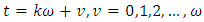
One of the most popular and frequently used stochastic time series models is the Autoregressive Integrated Moving Average (ARIMA) model. The basic assumption made to implement this model is to consider a time series model that is linear and follows a particular known statistical distribution, such as the normal distribution [1]. ARIMA model has a subclass of other models, such as the Autoregressive and Autoregressive Moving Average (ARMA) models. For seasonal time series forecasting, a Seasonal Autoregressive Moving Average (SARIMA) model is often used [2]. The popularity of the ARIMA model is mainly due to its flexibility to represent several varieties of time series with simplicity as well as the associated Box-Jenkins methodology for an optimal model-building process [3]. But the severe limitation of these models is the pre-assumed linear form of the associated time series which becomes inadequate in many practical situations. Recently, Artificial Neural Networks (ANNs) have attracted increasing attention in the domain of time series forecasting [4]. Although initially biologically inspired, but later on ANNs have been successfully applied in many different areas, especially for forecasting and classification purposes [5]. The excellent feature of ANNs, when applied to time series forecasting problems is their inherent capability of non-linear modelling, without any presumption about the statistical distribution followed by the observations. The appropriate model is adaptively formed based on the given data. Due to this reason, ANNs are data-driven and self-adaptive by nature [6]. During the past few years, a substantial amount of research work has been carried out towards the application of neural networks for time series modelling and forecasting. These include the works of [6] – [13]. For the capabilities of the ANN model discussed above, in this study, the ANN model based on multi-layer perceptrons (MLPs), which are characterized by a single hidden layer Feed Forward Network (FNN) will be considered for analysing climatic and economic variables that have been considered nonlinear according to [14].

Furthermore, [15] proposed a Fourier autoregressive model which is capable of modelling and forecasting time series that are presumed to exhibit seasonal and periodic variations simultaneously. Therefore, this study will be used to propose a multivariate form based on series decomposition into sine and cosine forms which usually reveal the periodicities in the time series. In essence, this study will model and forecast climatic variable that usually exhibits seasonality, periodicity and as well non-linear. Therefore, the traditional time series and Fourier-based models will be used to determine the best model for forecasting climatic variables when the series is considered to exhibit both seasonal and cyclical variation while the ANN model will be used to analyse the rainfall series that is presumed to be non -linear.

Improved rainfall forecasts benefit agriculture by enabling proactive farm management, optimizing irrigation, reducing losses from weather-related disasters, and allowing for better planning of planting and harvesting activities, ultimately leading to increased yields and reduced costs. Seasonal and long-term rainfall forecasts assist in planning for crop yields and managing water for irrigation. It affects ecosystems and biodiversity, planners use rainfall data to manage wetlands, riverine systems, and other natural resources. In disaster planning, improved rainfall forecasts enable early warnings, allowing communities to prepare and respond to potential disasters like floods and droughts, ultimately reducing loss of life and property damage. Based on the significant benefit of rainfall describe above, this study aims to model and forecast rainfall data that exhibit non-linearity, seasonality and periodicity simultaneously.

2. Literature Review

Univariate time series models are only one of the many methods used for forecasting and these models have been used in many fields. Akinwale et al., (2009) [16] used ARIMA and regression neural network with a back-propagation algorithm to analyze and predict translated and un-translated Nigerian stock market prices (NSMP). Their study compared the forecast performance of the neural networks with translated and un-translated NSMP as inputs, and this revealed that the network with translated NMSP inputs outperformed the network with un-translated NSMP inputs. In terms of prediction accuracy measures, the translated NSMP network predicted accurately 11.3% of the stock prices as compared to the 2.7% prediction accuracy of the un-translated NSMP network model. Ojo and Olatayo (2009) [17] studied the estimation and performance of subset autoregressive integrated moving average (ARIMA) models. They estimated parameters for ARIMA and subset ARIMA processes using numerical iterative schemes of Newton-Raphson and the Marquardt-Levenberg algorithms. The performance of the models and their residual variance was examined using AIC and BIC. The result of their study showed that the Subset ARIMA model outperformed the ARIMA model with a smaller residual variance. Emenike (2010) [18] studied the NSE market returns series using monthly data of the All-Share-Index for the period January 1985 through December 2008. In the study, an ARIMA (1,1,1) model was selected as a tentative model for predicting index points and growth rates. The results revealed that the global meltdown destroyed the correlation structure existing between the NSE All-Share-Index and its past values.

Liu et al., (2010) [8] determine that ANNs remain a better choice than many traditional methods when dealing with nonlinear problems and possess great potential for the study of global climate change and ecological issues. They stated that ANNs can resolve problems that other methods cannot. This is especially true for situations in which measurements are difficult to conduct or when only incomplete data are available. It is anticipated that ANNs will be widely adopted and then further developed for global climate change and ecological research. Adewole et al., (2011) [9] proposed an artificial neural network foreign exchange rate forecasting model (AFERFM) for foreign exchange rate forecasting. The proposed model was divided into two phases, namely: training and forecasting. In the training phase, a back-propagation algorithm was used to train the foreign Modelling and Evaluation Performances with Neural Network Using Climatic Time Series Data. This allowed them to construct models which possess very high forecasting accuracy in the short and medium term. For example, their air passenger demand model had a MAPE (Mean Absolute Percentage Error) of 0.34%. However, they noted that the performance of neural network models heavily depends on choosing an appropriate training set. Adebiyi et al., (2012) [19] studied stock prediction with data mining techniques which is one of the most important issues in finance being investigated by researchers across the globe. They presented a hybridized approach which combines the use of the variables of technical and fundamental analysis of stock market indicators for the prediction of the future price of the stock to improve on the existing approaches. The hybridized approach was tested with published stock data and the results obtained showed remarkable improvement over the use of only technical analysis variables. Also, the prediction from hybridized approach was found satisfactorily adequate as a guide for traders and investors in making qualitative decisions.

Isenah and Olubusoye (2014) [20] used their study to report empirical evidence that artificial neural network-based models apply to the forecasting of stock market returns. The Nigerian stock market logarithmic returns time series was tested for the presence of memory before the models were trained. The test showed that the logarithmic returns process is not random and that the Nigerian stock market is not efficient. Two artificial neural network-based models were developed in the study. These networks' out-of-sample forecast performance was compared with a baseline model. The results obtained in the study showed that artificial neural network-based models are capable of mimicking closely the log returns as compared to the based model. The out-of-sample evaluations of the trained models were based on the directional change metric respectively. Based on these metrics, it was found that the artificial neural network-based models outperformed the based model in forecasting future developments of the returns process. Another result of the study shows that instead of using extensive market data, simple technical indicators can be used as predictors for forecasting future values of the stock market returns given that the returns have the memory of their past. Ali & Cigizoglu (2013) [21] studied monthly runoff coefficients of seven southern large basins are calculated and modelled to forecast a holdout dataset by using univariate autoregressive integrated moving average (ARIMA), multivariate ARIMA (ARIMAX), and Artificial neural network (ANN) models. The applied traditional model performances are found insufficient since the characteristic behaviours of the time series of direct runoff coefficients are very complicated. Therefore, a new Hybrid approach is adopted by using the time series decomposition procedure and ANN. ARIMA, ARIMAX, ANN, and Hybrid models are compared with each other. Their results indicated that the newly generated Hybrid approach can be generalized to boost the prediction capability of ANNs in complicated time series data. It is seen that the new model captures the physical behaviour of the direct runoff coefficient time series. The semi-random spikes of the direct runoff coefficient series are approximated sufficiently. Panagiotis et al., (2014) [22] used NN's model to forecast 30-time series, ranging in several fields, from economy to ecology. The statistical approach to artificial neural network modelling developed in his study was compared with linear modelling and to other three well-known neural network modelling procedures: Information Criterion Pruning (ICP), Cross-Validation Pruning (CVP) and Bayesian Regularization Pruning (BRP). The findings show that the linear models outperform the artificial neural network models and albeit selecting and estimating much more parsimonious models, the statistical approach stands up well in comparison to other more sophisticated ANN models.

Several Fourier-related methods have been used to unveil hidden periodicities and analysis periodic relationships over the years. Bliss (1958) [23] used periodic regression to analyse cyclic phenomena in Biology and Climatology in which the length of the cycle was determined independently of the response. A sine wave model was used and an analysis of variance was used to determine how many terms to be retained in the sine wave model. The result obtained showed that the methods had the capability of identifying periodicities in biological and climatic series. But the method was computationally difficult, and too many terms were been identified by the analysis of variance.

Bartfari (2002) [24], applied periodic regression to some set of data and the method was based on the harmonic model for time series. The starting point of the method was harmonic analysis (Fourier analysis). The results were optimized in a multifold manner resulting in a model which was easy to handle and able to forecast the underlying data. The results provided were particularly better when compared to other methods in the research work and the models were free from limitations characteristic of other methods. He further stated that the calculated results are easy to interpret and use for further decisions. The method shown seems to be very effective and useful in modelling time series consisting of periodic terms. An additional advantage was the easy interpretation of the obtained parameters but the method does not have the capabilities to obtain the amplitude and phase. Christiansen et al., (2012) [25] used their work to discuss seasonal variation occurrence as a common feature of many diseases, especially those of infectious origin. Studies of seasonal variation contribute to healthcare planning and the understanding of the ethology of infections. An overview of statistical methods for the assessment and quantification of the seasonality of infectious diseases, as exemplified by their application to disease in Denmark in 1995-2011. Additionally, they discussed the conditions under which seasonality should be considered as a covariate in studies of infectious diseases. The methods considered range from the simplest comparison of disease occurrence between the extremes of summer and winter, through modelling of the intensity of seasonal patterns by use of a sine curve, to more advanced generalized linear models. All three classes of the method have advantages and disadvantages. The choice among analytical approaches should ideally reflect the research question of interest. Simple methods are compelling but may overlook important seasonal peaks that would have been identified if more advanced methods had been applied. Most studies suggest the use of methods that allow estimation of the magnitude and timing of seasonal peaks and valleys, ideally with a measure of the intensity of seasonality, such as the peak-to-low ratio. Seasonality may be a confounder in studies of infectious disease occurs when it fulfils the three primary criteria for being a confounder that is when both the disease occurrence and the exposure vary seasonally without seasonality being a step in the causal pathway. In these situations, confounding by seasonality should be controlled. This confounding makes the sine curve used in this research cumbersome and the estimation of coefficients expensive.

Andrea et al., (2013) [26], studied demand forecasting of the fashion textile industry operating with a large variety of short lifecycle products, deeply influenced by seasonal sales, promotional events, weather conditions, advertising and marketing campaigns, on top of festivities and socio-economic factors. At the same time, shelf-out-of-stock phenomena must be avoided at all costs. Given the strong seasonal nature of the products that characterize the fashion sector, this research was then used to highlight how the Fourier method can represent an easy and more effective forecasting method compared to other widely used methods. For this purpose, a comparison between the fast Fourier transforms algorithm and another two techniques based on moving average and exponential smoothing was carried out on a set of 4-year historical sales data of a €60+ million turnover medium to a large-sized Italian fashion company, which operates in the women's textiles apparel and clothing sectors. The results showed that the Fourier analysis method was a better forecast performance when compared on the bases of their mean square error and root mean square error with other methods used.

3. Methodology

3.1. Data

The monthly rainfall data utilized in this study was extracted from the Nigeria Meteorological Agency [27]. The data covers the period from January 1998 to December 2024, with monthly frequency. Climatic change can significantly impact rainfall pattern, leading to changes in intensity, increased variability and more extreme event like flooding and landslides. Policy changes significantly impacted the rainfall data in the context of climate change and food security while economic condition has affected the rainfall data in the context of water resources management, water infrastructure investment and agricultural practices.

In this study, missing climatic data, especially rainfall will be handle using rainfall forecasts and statistical techniques like mean or median imputation. Similar, outliers, which are data points deviating significantly from the mean, will be handled through data transformation.

3.2. Artificial Neural Network (ANN)

An artificial neural network (ANN) is an interconnected group of artificial neurons that has a natural property for storing experiential knowledge and making it available for use. This original perceptron model contained only one layer, inputs are fed directly to the output unit via the weighted connections. Although the perceptron initially seemed promising, it was eventually proved that the perceptron could not be trained to recognize many classes of patterns.

3.2.1. Multilayer Perceptron (MLP)

The Multilayer perceptron (MLP) model was derived and gradually became one of the most widely implemented neural network topologies. Multilayer perceptron means a feed-forward network with one or more layers of nodes between the input and output nodes. The MLP overcomes many limitations of the single-layer perceptron, their capabilities stem from the non-linear relationships among the nodes. Two important characteristics of the MLP are its nonlinear processing elements (PEs) which have a nonlinearity that must be smooth (the logistic function and the hyperbolic tangent are the most widely used), and their massive interconnectivity (that is, any element of a given layer feeds all the elements of the next layer).

The first or the lowest layer is an input layer where external information is received. The last or the highest layer is an output layer where the problem solution is obtained. The input layer and output layer are separated by one or more intermediate layers called the hidden layers. The nodes in adjacent layers are usually fully connected by a cyclic arc from a lower layer to a higher layer. The functional relationship estimated by the ANN can be written as

(1)

where are independent variables and is a dependent variable? In this sense, the neural network is functionally equivalent to a nonlinear regression model. On the other hand, for an extrapolative or time series forecasting problem, the inputs are typically the past observations of the data series and the output is the future value. The ANN performs the mapping function as

(2)

where is the observation at time t. Thus the ANN is equivalent to the nonlinear autoregressive model for time series forecasting problems. It is also easy to incorporate both prediction variables and time-lagged observation into one ANN model, which amount to the general transfer function model. Before an ANN can be used to perform any desired task, it must be trained to do so.

Training is the process of determining the arc weights which are the key elements of an ANN. The training input data is in the form of vectors of input variables or training patterns.

The total available data is usually divided into a training set (in-sample data) and a test set (out-of-sample or hold-out sample) and a training pattern consisting of a fixed number of lagged observations of the series. Suppose we have N observations in the training set and there is a need for one-step-ahead forecasting, then using an ANN with input nodes, this gives training patterns. The first training pattern will compose of as inputs and as the target output. The second training pattern will contain as inputs and as the desired output. Finally, the last training pattern will be for inputs and for the target output. If a multilayer perceptron has a linear activation function in all neurons, that is, a linear function that maps the weighted inputs to the output of each neuron, then it is easily proved with linear algebra that any number of layers can be reduced to the standard two-layer input-output. What makes a multilayer perceptron different is that some neurons use a nonlinear activation function which was developed to model the frequency of action potentials, or firing, of biological neurons in the brain.

The two main activation functions that are used here are both sigmoid and are described by

(3)

and

(4)

where is the output and is the level of training of the node (Neuron).

The former function is a hyperbolic tangent which ranges from -1 to 1, and the latter, the logistic function, is similar in shape but ranges from 0 to 1. Here is the output of the i^th node (neuron) and is the weighted sum of the input synapses. The multilayer perceptron consists of three or more layers (an input and an output layer with one or more hidden layers) of nonlinearly-activating nodes and is thus considered a deep neural network. Each node in one layer connects with a certain weight to every node in the following layer. Some people do not include the input layer when counting the number of layers and there is disagreement about whether should be interpreted as the weight from or the other way around.

Learning occurs in the perceptron by changing connection weights after each piece of data is processed, based on the amount of error in the output compared to the expected result. This is an example of supervised learning and is carried out through back-propagation, a generalization of the least mean squares algorithm in the linear perceptron.

The error in output node in the data point (training example) is represented by

(5)

where is the target value and y is the value produced by the perceptron. Then the corrections to the weights of the nodes based on those corrections minimize the error in the entire output, given by

(6)

3.2.2. Multilayer Perceptron Model

Based on the work of [10], a Multilayer perceptron model is proposed thus. Let the weight of the link from the neuron in the layer to the neuron in the layer then neuron in the layer is given by

(7)

where are respectively its output, activation function and bias.

3.2.3. Diagnostic Checking in ANN Model

Diagnostic checking is an essential step in evaluating the performance of an Artificial Neural Network (ANN). Calculating the Mean Absolute Error (MAE) to evaluate the model's accuracy, calculating the Mean Squared Error (MSE) to evaluate the model's accuracy and precision and calculating the root mean square percentage error (RMSPE) to evaluate the model's accuracy and precision. Model performance plots that involve plotting of the predicted values against the actual values to evaluate the model's accuracy is essential just like plotting the residuals against the predicted values or time to evaluate the model's performance. Other diagnostic check for ANN include using cross-validation techniques to evaluate the model's performance on unseen data and bootstrapping techniques to evaluate the model's performance and estimate the variability of the model's parameters.

3.3. Autoregressive Integrated Moving Average (ARIMA) Model

ARIMA model is a Univariate time series model that consists of an autoregressive polynomial, an order of integration and a moving average polynomial. The usual forms of and are written as

(8)

and

(9)

where and are the autoregressive and moving average parameters respectively. is the observed value at time and is the value of the random shock at time . It is assumed to be independently and identically distributed with a mean of zero and a constant variance ARMA model comprised of AR and MA models, in which the current value of the time series is defined linearly in terms of its previous values as well as current and previous error series.

The ARMA model is given in Equation (10) as

(10)

Equation (10) can be simplified by a backward shift operator to obtain

(11)

Equation (11) can therefore be expressed as where with and consecutive differencing.

3.3.1. Seasonal Autoregressive Integrated Moving Average (SARIMA) Model

The seasonal autoregressive integrated moving average was proposed by [2] and it was an extension of the autoregressive integrated moving average developed by [28]. The model will be used to reflect and obtain the features of seasonal variation in a given time series.

Generally, the time series utilizes a lag operator to process .

A seasonal ARIMA model may be written as:

(12)

in equation (12), is a lag operator defined as

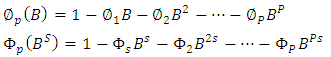(13)

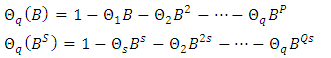(14)

where and are polynomials of order and respectively; and are polynomials in of degrees and , respectively; is the order of non-seasonal autoregression; is the number of regular differences; is the order of non-seasonal moving average; is the order of seasonal autoregression; is the number of seasonal differences; is the order of seasonal moving average; and is the length of the season, [29] – [30].

3.3.2. Model Building in Fourier Autoregressive (FAR)

The identification of the varying orders of FAR processes makes use of two similar functions, namely the periodic Autocorrelation function (PeACF) and periodic partial Autocorrelation function (PePACF). The choice of orders of the FAR model requires a detailed analysis of these functions respectively, whose shape and value determine the order of the model.

3.3.3. Periodic Autoregressive Function

For a univariate periodic stationary process were the white noise term are assumed to be independent, the periodic autocovariance function (PeACF) is defined as

(15)

For season at backward lag . Then the PeACF for period at back ward lag is defined as:

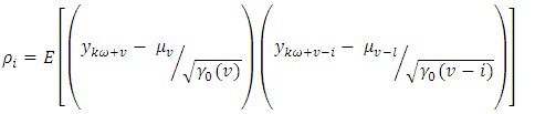(16)

(17)

where is the variance for the season and denote the periodically standardized time series, [15].

3.3.4. Sample Periodic Autocorrelation Function

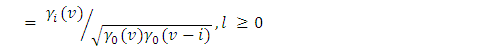
Let be a series of size (say, N years and periods) coming from a periodic stationary process Then the sample estimate of is called the sample periodic autocorrelation function given by;

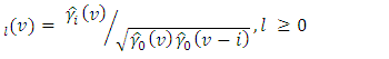(18)

where is the sample periodic autocorrelation function calculated from

(19)

In which

(20)

Is the sample mean for season .

3.4. Estimation of FAR Processes

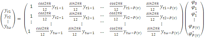
After the model identification, the Fourier autoregressive coefficients will be estimated using the discrete Fourier transform estimation method.

Let be the source of the periodic time series data and the discrete Fourier transform of the periodic stationary process is

(21)

If and then the periodic autoregressive coefficients of order for the seasons will be obtained as fellows

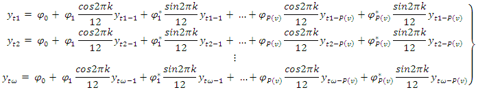(22)

In matrix form, we have it as

(23)

By taking the inverse of Equation (23), we have the Fourier autoregressive process coefficients.

To assess the correct order of the model fitted, the Akaike and Bayesian information criteria will be used. Akaike information criterion is given as

(24)

The optimal order of the model is chosen by the value of P for which AIC (P) is minimum.

Bayesian Information criterion is given by

(25)

where is the periodic estimator of and is the number of periodic autoregressive coefficients in the season, [15].

3.4.1. Diagnostic Checking in FAR Model

After parameter estimation, we will assess the model adequacy by checking whether the model assumptions are satisfied. The basic assumption is that the residuals are white noise. Hence a careful analysis of the estimated residuals will be carried out by checking whether the residuals are white noise and this is done by computing the sample ACF and PACF of the residuals to see whether they do not form any pattern and whether all are statistically significant, that is, within two standard deviation with . Other diagnostic checking in FAR includes plotting the residuals against time, fitted values, or other relevant variables to check for patterns or anomalies. Checking for autocorrelation in the residuals using plots or statistical tests, such as the Ljung-Box test and checking if residuals are normally distributed using plots or statistical tests, such as the Shapiro-Wilk test.

3.4.2. Forecasting in FAR Model

Given a FAR (1) model

(26)

(27)

where and is a constant.

Equation (26) can be written as

(28)

The general form of the forecast equation is given as

(29)

(30)

3.4.3. Forecast Evaluation for FAR Mode

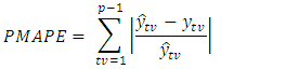
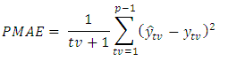
Once the forecast is made, an evaluation is computed to determine if the actual value of the series forecast is observed. There are some measurements of the accuracy of forecasts. These are Periodic root mean square error (PRMSE), Periodic Mean Absolute Error (PMAE) and Periodic Mean Absolute Percentage Error (PMAPE).

The periodic root means square error is defined as:

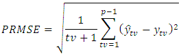(31)

the periodic mean absolute percentage error PMAPE is given as:

(32)

And the periodic mean absolute error PMAE is given as:

(33)

where The actual and predicted values for corresponding values are denoted by and respectively. The smaller the value of PRMSE, PMAPE and PMAE, the better the forecasting performance of the model, [15].

3.5. Models Justification

SARIMA model was employed in this study because it is a powerful time series tool for forecasting, particularly when dealing with data that exhibits both trend and seasonality. The Fourier Autoregressive (FAR) model is a powerful tool for time series analysis, particularly when dealing with data that exhibits periodic or cyclical patterns while the ANN model was used because of it effectively capture non-linear relationships between variables, which is common in many real-world applications.

4. Results

4.1. Time Series Model Building for the SARIMA Model

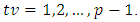
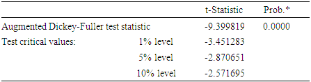
Table 1 provides the test for stationarity using the Augmented Dickey-Fuller test, the result indicates that the series is stationary at the 0.01 level of significance. In Table 2, the ACF and PACF tend to show a strong peak for the autocorrelation function, combined with peaks in the partial autocorrelation function. Hence, it appears that either: (i) the ACF is cutting off after lag 12 and the PACF is tailing off in the seasonal lags, (ii) the ACF and PACF are both tailing off in the seasonal lags. Table 2 suggests either (i) a seasonal moving average of order Q = 1, or (ii) because both the ACF and PACF may be tailing off at the seasonal lags, perhaps both components, P = 1 and Q = 1 are needed. To identify the between-season model, the focus is on the lags h = 1, 2…20. The ACF is tailing-off and the PACF is cut-off after lag 1, then p = 1 or 2 and q = 1 or 2. Also, it is possible to think of the PACF as tailing-off and the ACF as a cut-off after lag 1, leading to identify that P = 1 and Q= 1.

Table 1. Augmented Dickey-Fuller test result

Table 2. Autocorrelation and Partial Autocorrelation function for monthly rainfall

Based on this, the following four suggested models for the Nigerian monthly rainfall series are:

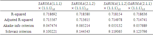
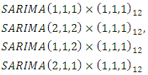The four suggested models were estimated using the ordinary least estimation method. The optimal model for rainfall will be chosen based on the smallest values of estimated Akaike information criteria (AIC), Schwarz information criteria and highest values of coefficient of determination and Adjusted coefficient of determination given in Table 3. The optimal model for Nigerian monthly rainfall is based on Table 3.

Table 3. The Combined SARIMA Results of the Rainfall Series

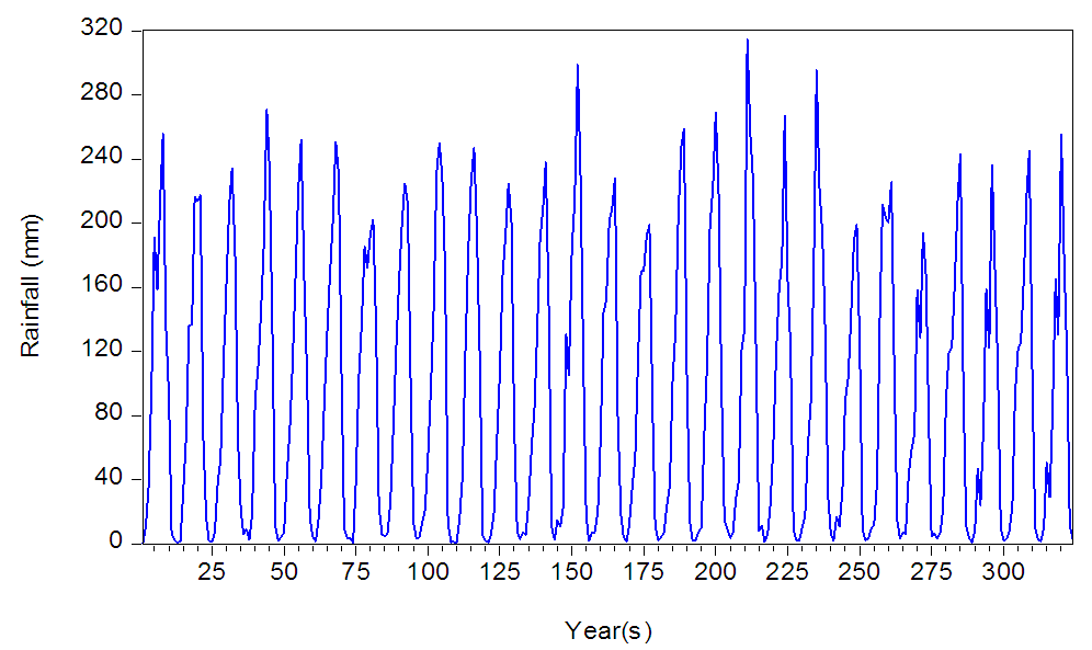Figure 1. Time plot of Nigerian monthly rainfall from January 1998 to December 2024

The diagnosis checking was done using Breusch and Pagan (B-P) test for the homoscedasticity of the residuals for the model. The results showed that all calculated values are found to be smaller than the respective critical values and this indicated that the residual variance is constant. Therefore, the hypothesis that the residuals are white noise cannot be rejected and this indicated the fitted model for rainfall and temperature series are adequate. That is, the model is adequate for modelling the Nigerian monthly rainfall series. The fitted model is used to obtain the forecast Nigerian monthly rainfall series from January 2025 to December 2026.

The fitted model for the rainfall series is expressed as;

(34)

Equation (34) can be re-expressed as:

(35)

To forecast one period ahead that is for the monthly rainfall series, Equation (35) will be increased by one unit throughout, and this will give

(36)

The forecasted values for the monthly rainfall series using Equation (36) are given in Table 4. This summarizes 24 months of up-front forecast from January 2025 to December 2026. The results showed a significant continuous rise and presence of seasonality in the forecasted rainfall time series data. In essence, there will be a rapid continuous increase in Nigerian rainfall value on monthly bases over the coming years. The result of the forecasting evaluation in Table 5 showed that all metrics used have relatively small and close to zero values. Hence, this indicated that the forecasting inaccuracy is very low.

Table 4. Nigerian monthly rainfall forecast with SARIMA model from January 2025 to December 2026

Table 5. Forecasting evaluation for the SARIMA model

4.2. Time Series Model for Fourier Autoregressive Model

The Fourier Autoregressive Model construction involves model identification, estimation, diagnosis and forecasting. The model identification will depend on periodic autocorrelation and partial autocorrelation function, and estimation will be based on discrete Fourier transformation to ordinary least square estimation method. The diagnosis will be based on the autocorrelation of the residuals while prediction will be done using eventual forecast.

4.2.1. Model Identification and Selection for Fourier Autoregressive Model

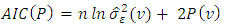
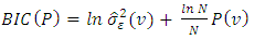
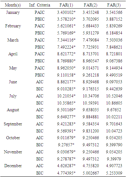
A critical look at the periodic autocorrelation and partial autocorrelation function showed that the periodic autocorrelation function was stable and period partial autocorrelation cut off at lag 2, so tentative FAR(1), FAR(2) and FAR(3) was considered. After the estimation of the tentative models, the information criteria, that is, Periodic Akaike Information Criterion (PAIC), and Periodic Bayesian Information Criterion (PBIC) has the smallest values in the FAR(1) model and this reason was used to choose FAR(1) as the better model based on the result in Table 6.

Table 6. Information Criteria for FAR models

4.2.2. Estimation and Diagnosis for Fourier Autoregressive Model

The FAR(1) models fitted for January to December are given in equation (37) and their residual errors were diagnosed using periodic residual autocorrelation. The periodic residual autocorrelation for FAR(1) showed the residual was white noise, hence the models can be used to forecast Nigerian monthly rainfall series.

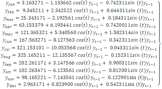(37)

where

4.2.3. Forecast and Forecast Evaluation of Fourier Autoregressive Model

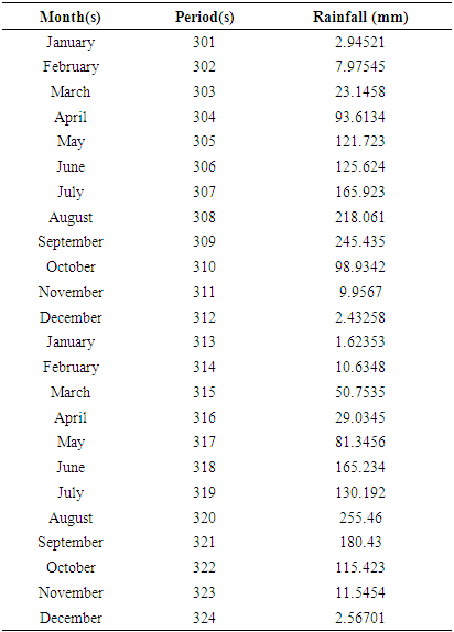
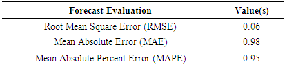
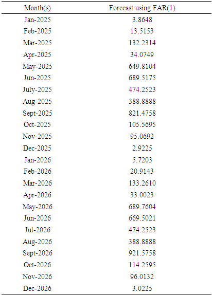
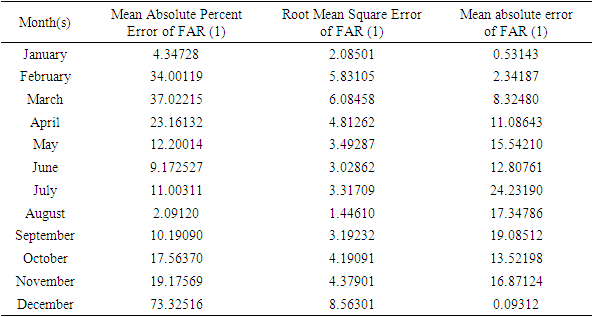
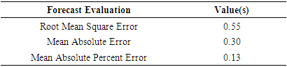
Out-sample forecasts were obtained for the Nigerian monthly rainfall series based on the FAR(1) models. The in-sample forecast for January to December showed a close look at the original series and the out-sample forecast in Table 7 showed a consistent and close reflection of the original series from January 2025 to December 2026. The values of the forecast evaluation in Table 8 showed the forecast was consistent since their values were relatively low.

Table 7. Forecasting result of Fourier Autoregressive Model

Table 8. Forecast Evaluation of Nigerian Rainfall Series from Jan. 2025 to Dec. 2026

4.3. Artificial Neural Network (ANN) Model Analysis

The ANN analysis was based on multilayer perception and Nigeria's monthly rainfall series is used as the dependent variable while temperature and evaporation were used as factors and covariates respectively.

4.3.1. Monthly Rainfall Series with ANN Based on Multilayer Perception

Since the climatic variables are not obtained based on the same measurement then the covariate will be rescaled by using the method of standardization by subtracting from the mean and dividing by the standard deviation that is

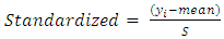(38)

The first stage in multilayer perception is to partition the dataset and randomly assign cases based on the relative number of cases and specify the relative number (ratio) of cases to each sample that is training, testing, and holdout. Here 7, 3, and 0 are specified as the relative numbers for training, testing, and holdout samples corresponding to 70%, 30%, and 0% respectively.

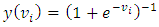In the architecture stage, two hidden layers were considered and the activation function will be based on the sigmoid given as; and it takes real-valued arguments and transforms them to the range (0, 1).

The training stage was used to determine how the network processes the records. The batch training method is adopted since it can update the synaptic weights only after passing all training data records; that is, batch training uses information from all records in the training dataset and it is preferred because it directly minimizes the total error and the optimization algorithm.

Table 9. Case Processing summary of artificial neural network

Table 10. model summary of Artificial Neural Network

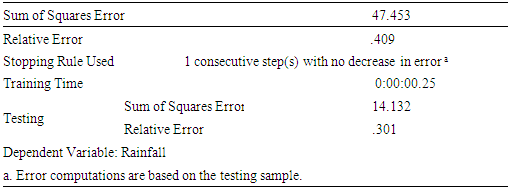
4.3.2. Interpretation of the ANN based on Multilayer Perceptron

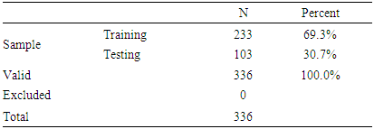
ANN based on multilayer perceptron result show that 233 observations are trained and 103 observations are tested and this implies that 233 observations are valid. This shows that 69.3% of the observations input are trained and 30.7% are tested. The rainfall prediction from the ANN model to multilayer perception shows a slightly perfect match to the original data. The forecast performance evaluations in Table 11 for ANN based on the multilayer perception model are relatively low.

Table 11. Forecasting evaluation for ANN based on multilayer perception model

5. Discussion

In this study, three different models that is, SARIMA, FAR and ANN based on Multilayer Perceptron models were employed to model and forecast Nigerian monthly rainfall series. This study focused on climatic variables that usually exhibit seasonality, periodicity and as well as non-linearity. Therefore, the traditional time series and Fourier-based models were used to determine the better model for forecasting climatic variables when the series is considered to exhibit both seasonal and cyclical variations while ANN based on the Multilayer Perceptron model was used to analyze the rainfall series that is presumed to be non -linear.

SARIMA model characteristics, including the orders for non-seasonal components and for seasonal components, and the seasonal period (12), significantly impact estimation performance. The study carefully selected the model and parameter which is crucial for accurate forecasting. Fourier Autoregressive (FAR) model characteristics, especially the order of the autoregressive (AR) component and the number of Fourier terms, such as FAR (1), FAR (2) and FAR (3) used in this study, significantly impacted the estimation and forecast performance, with higher orders potentially capturing more complex patterns. The estimation and forecasting performance of Artificial Neural Network (ANN) models was significantly influenced by the architecture used, including the number of layers, neurons, and the type of activation functions used, as well as the training algorithms and rainfall dataset that was utilized in the study.

From the results of the study, the time plot showed that Nigerian monthly rainfall is non-stationary and exhibits seasonal, cyclical variations and as well it is non-linear. Augmented Dickey fuller test was employed to test for stationarity, the series was stationary at the first difference that is, d =1. The autocorrelation and partial autocorrelation were used to determine the presence of seasonality and 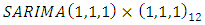was identified as the best model based on AIC and BIC values. The model was estimated and diagnosed using the least square method and Breusch and Pagan (B-P) test for the homoscedasticity of the residuals respectively. The SARIMA model was used to obtain a forecast for Nigeria's monthly rainfall based on forecast evaluation metrics like, MAE, RMSE and PMAE.

Fourier autoregressive model which involved model identification, estimation and diagnostic checking and forecasting was employed to model the Nigerian monthly rainfall in the context of seasonality and periodicity variation present in the series. From the results, Fourier autoregressive, FAR (1) was identified for January to December periodic rainfall series using sample periodic autocorrelation and partial autocorrelation functions. The January to December fitted models in the equation were all validated using the values of PAIC and PBIC. To check the stability of the fitted model, a residual autocorrelation plot was used to show that the error terms were white noise. The validated periodic models were used to obtain an out-sample forecast while the out-sample forecast exhibited fluctuations from January 2025 to December 2026. The forecast was validated using the following forecast evaluations, MAE, RMSE and PMAE.

ANN based on multilayer perception was used to model and predict Nigeria's monthly rainfall in the context of non-linearity. The result showed that 233 observations are trained, and 103 observations are tested and this implies that 233 observations are valid. This shows that 69.3% of the observations input are trained and 30.7% are tested. Prediction from the ANN model with respect to multilayer perception shows a slightly perfect match to the original data. The forecast performance evaluations for ANN based on a multilayer perception model were utilized to validate the forecast.

To check the efficiency of the models that were used to forecast Nigeria's monthly rainfall based on the forecast performance evaluations (MAE, RMSE and PMAE) of the SARIMA, FAR and ANN models, there is an indication that the FAR model outperforms the SARIMA model when considering time series that exhibit both seasonal and cyclical variation simultaneously based on the forecasted values and their forecast performance evaluations while Artificial Neural Network based on multilayer perceptron will be considering when the non-linear characteristics of Nigeria monthly rainfall series are put in forward based on the model forecast performance evaluations.

6. Conclusions

The complexity of the nature of rainfall time series data as a factor for climatic change with evidence of seasonality, periodicity and non-linearity has been studied using SARIMA, ANN and FAR models. The study reveals that in the context of non-linearity, the artificial neural network is appropriate. In the context of stationarity and seasonality, Seasonal Autoregressive Integrated Moving Average is suitable while the FAR model is appropriate when seasonality and periodicity are of main concern. Conclusively, this study has been used to establish the presence of seasonality, periodicity and nonlinearity variations simultaneously in Nigeria's monthly rainfall data. In essence, SARIMA, FAR and ANN models are all useful models when modelling and forecasting Nigeria's monthly rainfall time series data. The ever-changing situation in our immediate environments has caused a lot of changes in the structure and pattern of time series data over the years which make it often cyclic. Therefore, analyzing this requires the construction of efficient and better statistical analysis methods which will give room for proper and correct statistical inference that leads to drawing valid decisions and conclusions.

Based on the findings, it is recommended that the ANN model can be used as an appropriate forecasting tool to forecast rainfall when non-linearity is of interest, while the FAR model will be the appropriate model for forecasting rainfall series when seasonality and periodicity are of the main concern. Therefore, our study established that SARIMA, FAR and ANN models are all appropriate models that can be combined to model and forecast rainfall data to provide results that can help in combating climatic change. The methods used in this study for analyzing time series data variation may be far from being exhaustive. However, the results will enhance further work that will be carryout using the same data set by extending the Fourier Autoregressive model into Bivariate Fourier Autoregressive or hybrid of ANN and FAR model which can be used to model and forecast multiple time series data that are seasonal and periodic simultaneously.