-
Paper Information
- Paper Submission
-
Journal Information
- About This Journal
- Editorial Board
- Current Issue
- Archive
- Author Guidelines
- Contact Us
International Journal of Statistics and Applications
p-ISSN: 2168-5193 e-ISSN: 2168-5215
2024; 14(4): 65-73
doi:10.5923/j.statistics.20241404.01
Received: Sep. 28, 2024; Accepted: Oct. 22, 2024; Published: Oct. 30, 2024

Parameter Inference of Transmuted Power Lomax Distribution
 Abstract
 Reference
 Full-Text PDF
 Full-text HTML
Ahmed Hurairah, Mohammed Al-Maweri
Department of Statistics, Sana’a University, Sana’a, Yemen
Correspondence to: Ahmed Hurairah, Department of Statistics, Sana’a University, Sana’a, Yemen.
| Email: |  |
Copyright © 2024 The Author(s). Published by Scientific & Academic Publishing.
This work is licensed under the Creative Commons Attribution International License (CC BY).
http://creativecommons.org/licenses/by/4.0/

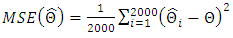
The main purpose of the paper is to investigate the inferences for the unknown parameters of the transmuted Power Lomax (TPL) distributionproposed by Moltok [25]. Maximum likelihood (ML) method is used to estimate the unknown parameters of TPL distribution. A simulation study evaluating the performance of the maximum likelihood estimators is conducted and a comparison of performance is made. The Likelihood Ratio (LR) and Wald (W) tests are derived for testing the null hypothesis. A simulation study evaluating the performance of the (LR) and (W) test statistics in terms of their size and power in testing hypothesis of the parameters of the TPL distribution. Moreover, the confidence intervals of the parameters of transmuted Power Lomax (TPL) distribution based on likelihood ratio and Wald statistics are evaluated and compared through the simulation study. The criteria used in evaluating the confidence intervals are the attainment of the nominal error probability and the symmetry of lower and upper error probabilities.
Keywords: Transmuted Power Lomax distribution, Maximum likelihood estimation, Likelihood ratio test, Confidence interval, Coverage probability, Simulation
Cite this paper: Ahmed Hurairah, Mohammed Al-Maweri, Parameter Inference of Transmuted Power Lomax Distribution, International Journal of Statistics and Applications, Vol. 14 No. 4, 2024, pp. 65-73. doi: 10.5923/j.statistics.20241404.01.
Article Outline
1. Introduction
- The Lomax distribution proposed by Lomax [23] as a kind of Pareto-II was introduced originally for modelling business data and has been widely applied in a variety of contexts, thanks to its flexibility. Many authors have proposed extensions of the Lomax distribution and the three-parameter continuous distribution which we have power Lomax (PoLo) distribution developed by El-Houssainy et Al. [13], is one of them. Power Lomax distribution accommodates both decreasing and inverted bathtub hazard rate that is required in various survival analysis. In the literature, there are several extensions of the Lomax distribution, these among others include the weighted Lomax distribution by Kilany [18], exponential Lomax distribution by El-Bassiouny et al. [12], exponentiated Lomax distribution by Salem [29], transmuted Lomax distribution by Ashour and Eltehiwy [4], Poisson Lomax distribution by Al-Zahrani and Sagor [3], Weibull Lomax distribution by Tahir et al. [32], power Lomax distribution by Rady et al. [28], Mar-shall–Olkin extended-Lomax by Ghitany et al. [14] and Gupta et al. [15], Beta–Lomax, Kumaraswamy Lomax, McDonald-Lomax by Lemonte and Cordeiro [22], Gam-ma-Lomax by Cordeiro et al. [7] and Exponentiated Lo-max by Abdul-Moniem [2]. The cdf and pdf of the transmuted Power Lomax distribution are obtained using the steps proposed by Shaw and Buckley [31]. A random variable X is said to have a transmuted distribution function if its pdf and cdf are respectively given by;
 | (1) |
 | (2) |
 is the transmuted parameter, G(x) is the cdf of any continuous distribution while f(x) and g(x) are the associated pdf of F(x) and G(x), respectively. Recently, various generalizations have been introduced based on the transmutation map approach. Moltok et al. [25] proposed the transmuted Power Lomax distribution as an extension of the popular Lomax distribution in its power transformation-form using the Quadratic rank transmutation map. The pdf of the transmuted Power Lomax distribution is defined by
 | (3) |
 | (4) |
 The work in this paper is concerned with the investigation of the parameters inference for the transmuted Power Lomax distribution. The maximum likelihood estimator of the parameters of transmuted Power Lomax distribution is not available in closed form. Thus, a simulation study is conducted to investigate the bias, finite sample variance (FSV), and the mean square error (MSE) of the maximum likelihood estimator of the parameters of the transmuted Power Lomax distribution. The adequacy of variance estimates obtained from the inverse of the observed information matrix is also considered. Exact testing hypothesis procedures for the transmuted Power Lomax distribution are intractable. Therefore, two standard large sample statistics based on maximum likelihood estimator were considered, which are the likelihood ratio and the Wald statistics. Their performances in finite samples in terms of their sizes and powers are investigated and compared. Confidence intervals based on the likelihood ratio and the Wald statistics were studied. The performances in terms of the attainment of the nominal error probability and symmetry of lower and upper probabilities were investigated and compared. The rest of this paper is organized as follow: Section 2 presents the parameter inference for the transmuted Power Lomax (TPL) distribution. A simulation study evaluating the performance of the maximum likelihood estimators and the size and power of the LRT and Wald are compares. Another simulation study evaluating the accuracy of approximate confidence intervals for the four-parameter of the TPL distribution. The conclusion is reported in Section 3.
2. Parameter Inference
- Inference can be carried out in three different ways: point, interval estimation and hypothesis testing. Several approaches for parameter point estimation were proposed in the literature but the maximum likelihood method is the most commonly employed. The MLEs enjoy desirable properties and can be used in testing statistics. Large sample theory for these estimates delivers simple approximations that work well in finite samples. Statisticians often seek to approximate quantities such as the density of a test statistic that depend on the sample size in order to obtain better approximate distributions. The resulting approximation for the MLEs in distribution theory is easily handled either analytically or numerically. So, we consider the estimation of the unknown parameters of the TPL distribution by the method of maximum likelihood.
2.1. Parameter Estimation
- Suppose
 be a random sample consisting of
  observations from the four-parameter transmuted Power Lomax distribution. Let
  be the vector of the parameters. Then the log-likelihood function for the vector of parameters
  can be expressed as
  | (5) |
 and
and  then equating it to zero, we obtain the component of the score vector
  is given by
 | (6) |
 | (7) |
 | (8) |
 | (9) |
 of the unknown parameters
  respectively, can be obtained by setting the score vector to zero and solving the system of nonlinear equations simultaneously. Since there is no closed form solution of these non-linear system of equations, we can use numerical methods such as Newton-Raphson type algorithms to numerically optimize the log-likelihood function to get the maximum likelihood estimates of the parameters
  To compute the standard error and the asymptotic confidence interval, we use the usual large sample approximation in which the maximum likelihood estimators for
  can be treated as being approximately normal. For a random sample
  of size
  from
from  distributed with pdf (3), the sample log-likelihood is
  , where
  is the log-likelihood for the
  observation
  and the score vector is
 The maximum likelihood estimate (MLE)
  of
of  is obtained by solving the system
 Under certain regularity conditions,
  , (here
  stands for convergence in distribution), where
  denotes the information matrix given by
 This information matrix
  may be approximated by the observed information matrix
 Then, using the approximation,
  , one can carry out tests and find confidence regions for functions of some or all parameters in
  .
.2.1.1. Simulation Study
- Here, we assess the finite sample behaviors of the MLEs for the four-parameter TPL distributions. The assessment of the finite sample behavior of the MLEs for this distribution was based on the following:1. Use the inversion method to generate two thousand samples of size n from the TPL distribution, i.e. generate values of:
 | (10) |
 for
for  3. Compute the bias, finite sample variance (FSV) and mean squared errors (MSE) for two thousand samples. The finite sample variance (FSV) are computed by inverting the observed information matrix. Bias and MSE are given by:
 | (11) |
 | (12) |
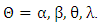 4. We repeat these steps 2000 times (iteration) for n= 10, 40, 70, 100, 150, 200, and 300, so computing
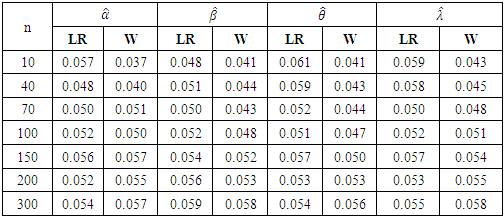
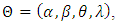
 The average estimates, along with the bias, mean squared error and finite sample variance are presented in Table 1.
|
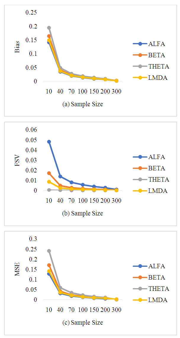 | Figure 1. Relationship between the bias (a), FSV (b) and MSE (c) of the estimators and sample size |
2.2. Testing Hypothesis
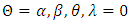
- For the four-parameter TPL distribution given in (6), we shall consider testing the null hypothesis,
 with the alternative
  . For testing
  versus
  , two commonly used tests based on the statistics proposed by Neyman and Pearson that is the likelihood ratio statistic [26] and Wald [35] are employed. For the likelihood ratio and Wald tests of
  versus
  , one needs the maximum likelihood estimators of
  under
under  . The likelihood ratio test statistic for testing
  versus
  is
is | (13) |
 versus
  is
is | (14) |
 and
and  are the MLEs under
  and
and  the inverse of one of the parameters section of the matrix of the second partial derivatives evaluated at
  The statistic
  and
and  are asymptotically (as n → ∞) distributed as
  where r is the dimension of the subset Ω of interest. The likelihood ratio and Wald tests rejects
  if
if  In practice with various sample sizes, the powers of these tests differ, and the relative performance of the test changes from model to model (Lawless, 1982). Since it is of utmost important to use the test with highest possible power, it is necessary to apply these tests using finite sample to get a better understanding of the process. To investigate the performance of the likelihood ratio and Wald tests, we shall compare the size and the power of the likelihood ratio and Wald test statistics. Size of the test is determined as the number of rejections of the null hypothesis divided by the total number of replications, (Abood and Young, [1]). The Size of the test is given by
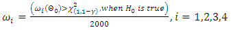 | (15) |
 The power of the test at a given
  in the parameter space is computed as the number of rejections of the null hypothesis given that the true value of the parameter is
  . The Power of the test is given by
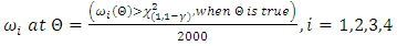 | (16) |
2.2.1. Simulation Study
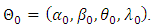
- In this simulation study, the level of significance taken is 0.05 and the sample size chosen are 10, 40, 70, 100, 150, 200 and 300. We then compare the size and the power of the two test statistics with the various sample sizes. The value specified by the null hypothesis is
 . The results of the simulation are given in Tables 2 and 3. The results concerning the size of the tests for the estimator are given in Table 2. The results on the power performance of the tests for the estimators are given in Table 3.
|

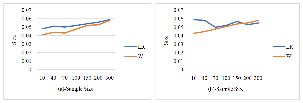 | Figure 2. Size of the likelihood ratio and Wald test statistics for testing β (a) and λ (b) parameters when γ = 0.05 |
 Likelihood Ratio and Wald tests perform well for all sample size.
|

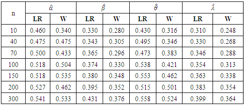
 | Figure 3. Power of the likelihood ratio and Wald test statistics for testing α (a) and θ (b) parameters when γ = 0.05 |
2.3. Confidence Intervals
- Exact interval estimates for the TPG distributions is difficult to obtain. Consequently, large sample intervals based on the asymptotic maximum likelihood estimators have gained widespread use. Asymptotic normal theory for the maximum likelihood estimators provides easily computable approximate confidence intervals. Many studies have been taken on the interval estimation, Hurairah et al. [16] studied the confidence intervals of the parameters of the new extreme value distribution based on likelihood ratio, Wald and Rao statistics and compared through the simulation study. The criteria used in evaluating the confidence intervals are the attainment of the nominal error probability and the symmetry of lower and upper error probabilities. Mann and Ferting [24]; discussed the estimation functions for parameters of the extreme value and two-parameter Weibull distributions that are fully efficient. Doganaksoy and Schmee [9,10] evaluated the accuracy of asymptotic normal intervals and likelihood ratio-based intervals. For the smallest extreme value and normal distributions under various degrees of censoring and to assess the extent to which square root of the likelihood ratio statistic and Bartlett corrections achieve their goals. Let
 be a sample from a distribution with joint log-likelihood function
  , where
  is a parameter of interest, and
  is a vector nuisance parameter. Two widely used methods for inference concerning
  are based on the likelihood ratio statistic and Wald statistic. It is well known that the overall maximum likelihood estimator,
  , is asymptotically distributed as normal distribution with mean
  and its asymptotic variance can be estimated by the inverse of either the expected Fisher information matrix or the observed information matrix evaluated at
  . Hence, a
  confidence interval for
  based on the likelihood ratio statistic is
 | (17) |
 is the log-likelihood function of
  is the overall maximum likelihood estimator of
  and
and  is the restricted maximum likelihood estimator of
  given a fixed value of
  . Under usual regularity conditions, the likelihood ratio statistic
  has an asymptotic chi-square distribution with one degree of freedom (Cox and Hinkley, [8]). Under usual regularity assumptions on the likelihood function, the lower
  and upper
  confidence limits are the two values of
  that satisfy
 Alternatively, it is also well known that the Wald statistic
 | (18) |
 is the
  percentile of N (0, 1).We describe the simulation study to evaluate and compare the performance of the confidence intervals of the parameters for finite sample. The criterion that we use as a basis of our study is the attainment of the nominal error probability and the symmetry of the lower and upper tail probabilities (Jennings, [17]). Attainment of the nominal error probability is important because otherwise we use an interval with an unknown coverage probability and our conclusions therefore are imprecise and can be misleading. The other criterion is the symmetry of the lower and upper error probabilities, that is, if the intervals fail to contain the true value of the parameter, it is equally likely to be above or below the true value. The use of two-sided confidence intervals expects this symmetry because they are using symmetric percentiles of the approximating distribution that has been used to form the confidence intervals. However, symmetry of error probabilities may not occur due to the skewness of the actual sampling distribution. The criterion used in evaluating the confidence intervals under this study is the attainment of the nominal error probability and the symmetry of lower and upper error probabilities. The standard errors of an estimated actual error probability rates at a given nominal error level
  is approximately:
 | (19) |
 is the number of replications,
  is the nominal error probability, assuming that the observed error rates are close enough to the nominal (see Doganaksoy and Schmee, [11]). The nominal level is attained if the observed total error probability is contained in the interval
  . If the total error probability is greater than
  , then the method of interval is termed anticonservative. However, if the total observed error probability is less than
  , then the method is termed conservative. If the total observed error probability attains the nominal level, then the method of interval estimation gives symmetric lower and upper probabilities when the larger error is not greater than (1.5) times the smaller one (Doganaksoy and Schmee, [9,11]). The lower, upper, and the total error probabilities were obtained for the likelihood ratio and Wald statistics based on confidence intervals with 0.05 for the parameters. Lower and upper error probabilities of a
  confidence interval based on the likelihood ratio statistics for the parameters are given respectively by (Doganaksoy, [10])
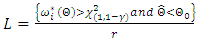 | (20) |
 | (21) |
 confidence interval based on the Wald statistics for the parameters are given respectively by
  | (22) |
 | (23) |
2.3.1. Simulation Study
- In this simulation, the level of significance is taken as 0.05, and the sample size is taken as 10, 40, 70, 100, 150, 200 and 300 to compute two-sided
 confidence intervals based on the likelihood ratio and Wald statistics are then computed. Table 4, contains, lower error probability (L), upper error probability (U) and total error probability (T) of the likelihood ratio intervals with sample size n=10,40,70,100,150,200 and 300 when
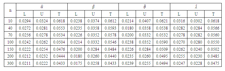 | Table 4. Lower, Upper, and Total Error Probabilities of 95% confidence limits Based on the Likelihood Ratio for the parameters of TPL distribution |
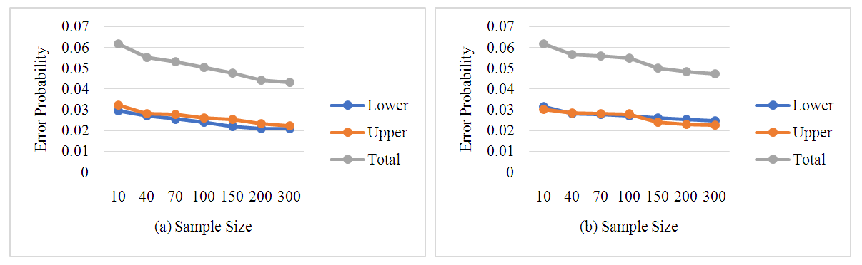 | Figure 4. Error probability of likelihood ratio intervals for the α (a) and λ (b) parameters when γ = 0.05 |
 when
when 
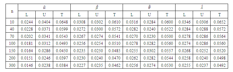 | Table 5. Lower, Upper, and Total Error Probabilities of 95% confidence limits Based on the Wald for the parameters of TPL distribution |
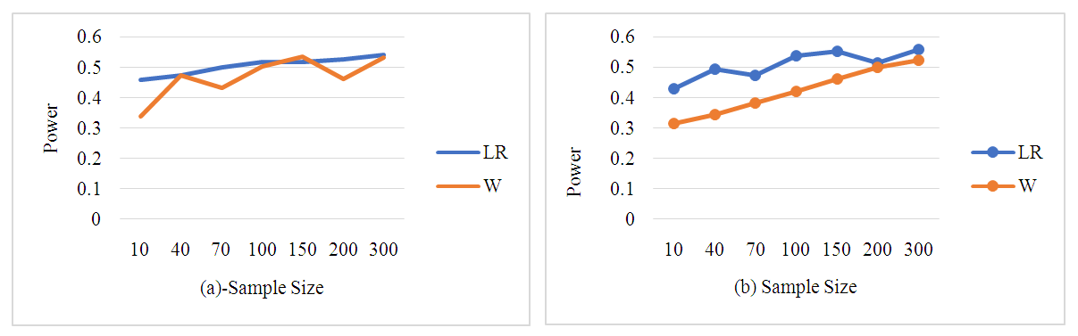
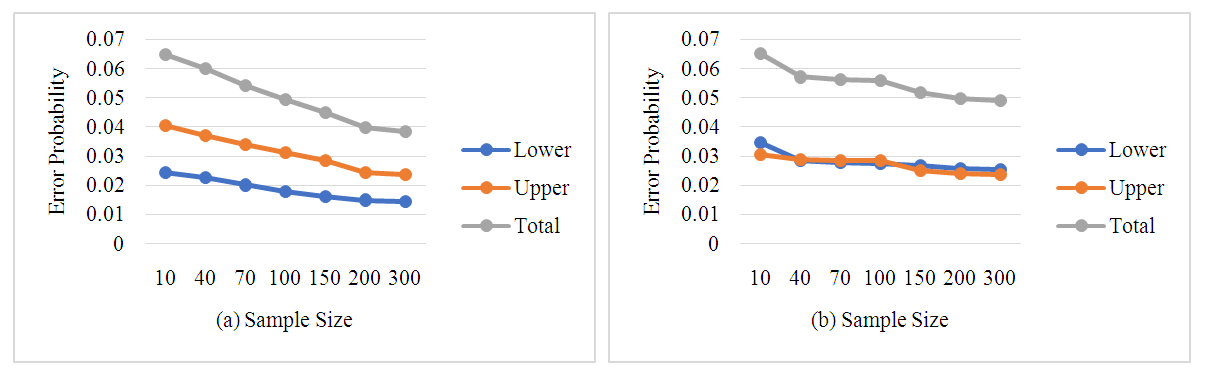 | Figure 5. Error probability of Wald intervals for the α (a) and λ (b) parameters when. γ = 0.05 |
 The total error probability for all parameters attained the nominal level. Table 5 shows that as the sample size increases, the average confidence lengths decrease and for the
  parameters, the intervals appear to have highly symmetric lower and upper error probabilities, especially for small sample size when n=10. These intervals tend to have a total error probability that is slightly higher than the nominal, while it is nominal when sample size greater than 10. For small sample size (n=10), the intervals tend to be anticonservative, as shown in Table 5. For the
  parameters, the intervals tend to be symmetric for all sample sizes, and they generally attain the nominal level.
 3. Conclusions
- The paper is concerned with the investigation of the finite sample performance of asymptotic inference procedures using the likelihood function based on the TPL distributions. The study includes investigating the adequacy of asymptotic inferential procedures in small samples. The maximum likelihood estimator of the parameters of TPL distributions is not available in closed form. Thus, a simulation study is conducted to investigate the bias finite sample variance (FSV), and the mean square error (MSE) of the maximum likelihood estimator of the parameters of the TPL distribution. Exact testing hypothesis procedures for the TPL distribution are intractable. Therefore, two standard large sample statistics based on maximum likelihood estimator were considered, which are the likelihood ratio and the Wald statistics. Their performances in finite samples in terms of their sizes and powers are investigated and compared. Confidence intervals based on the likelihood ratio and the Wald statistics were studied. The performances in terms of the attainment of the nominal error probability and symmetry of lower and upper probabilities were investigated and compared. The main findings of the simulation studies of the inference procedures for the parameters of the TPL distribution indicate that the estimate of the parameter’s performance satisfactory in terms of bias and variance in all the situations considered. In the hypothesis testing of the TPL distribution, the likelihood ratio statistic appears to perform better than the Wald statistics. Interval estimates for the scale parameter based on Wald statistic is highly symmetric and tend to be slightly anticonservative, while intervals based on the likelihood ratio statistics are in general symmetric and attain the nominal error probability. Likelihood ratio based intervals perform much better than the Wald intervals.