Ilesanmi A. O.1, Halid O. Y.1, Adejuwon S. O.2, Odukoya E. A.1, Olayemi M. S.3
1Department of Statistics, Ekiti State University, Ado-Ekiti, Ekiti State, Nigeria
2Department of Mathematical and Physical Sciences, Afe Babalola University, Ado Ekiti, Nigeria
3Department of Statistics, School of Applied Sciences, Kogi State Polytechnic, Lokoja
Correspondence to: Adejuwon S. O., Department of Mathematical and Physical Sciences, Afe Babalola University, Ado Ekiti, Nigeria.
| Email: |  |
Copyright © 2024 The Author(s). Published by Scientific & Academic Publishing.
This work is licensed under the Creative Commons Attribution International License (CC BY).
http://creativecommons.org/licenses/by/4.0/

Abstract
This work focused on the performance evaluation of some estimators of generalized extreme value distribution. The location, scale and shape parameters of the generalized extreme value distribution was estimated using four estimating methods, namely, the maximum likelihood, L-moments, TL-moments (1,0) and TL-moments (1,1). Instead of simulating data which is common in the literatures the GEV distribution is fitted to annual maximum rainfall measurements obtained from Nigeria metrological agency (NIMET) from 1980-2021. The results of estimates and mean square error was calculated using computer programming language R and R studio. The estimation technique which yielded the smallest mean square error was selected as the best performing estimator. The results show that the TL-moments (1,1) gave the least mean square error (MSE) value in Ekiti and Ondo. This indicates that TL-moments (1,1) is the most efficient estimator in the two selected states in south western zone of Nigeria considered in this work, while the MLE is the least efficient estimator with the highest mean square error. Also, the estimation of return level by different methods increases as the return period increases.
Keywords:
Generalized Extreme value Distribution, Rainfall, Nigeria metrological agency, Maximum likelihood, Mean square error
Cite this paper: Ilesanmi A. O., Halid O. Y., Adejuwon S. O., Odukoya E. A., Olayemi M. S., On the Performance Evaluation of Some Estimators of Generalised Extreme Value Distribution, International Journal of Statistics and Applications, Vol. 14 No. 2, 2024, pp. 35-40. doi: 10.5923/j.statistics.20241402.03.
1. Introduction
The generalized extreme value distribution is a three-parameter distribution that combines the Gumbel, Fréchet, and Weibull distributions into a single framework. Jenkinson (1955) introduced the generalized extreme-value (GEV) distribution which has been used in many research fields, for instance, Zelina et al. (2002) analysed annual maximum rainfall series in Malaysia and Bangladesh using eight probability distributions, they showed that generalised extreme value (GEV) is the suitable distribution to describe data in Malasia and Bangladesh. Also, Zin and Jemain (2010) used GEV in statistical distributions of yearly intense sequence and part moisture less series of drought occasion between 1975-2004 in Malaysia. In finding the best model to fit flood events of the Pachang river in Taiwan, Nadarajah and Shiau (2005) applied the Gumbel and GEV distributions as models of extreme values and showed that the Gumbel distribution can be considered over the GEV distribution for both flood volume and flood peak. Gamage et al (2009) considered a series of annual maximum rainfall and found that GEV is the most suitable distribution. Park et al. (2010) also identified GEV as the best fit probability density function (PDF) for frequency analysis of annual maximum daily rainfall events in South Korea. There are various methods used in parameter estimation of generalized extreme value distribution such as maximum likelihood method, maximum spacing product (MPS) method, L-moment, Probability weighted moment, TL-moments and Bayesian. In many cases GEV parameters are generally estimated using most widely accepted estimation method (maximum likelihood) due to it favourable property like its asymptotically normal property. Hosking et al (1985) showed that MLE method usually performed very well when the sample sizes become very large however it may not be the best when the sample sizes are small. Similarly, Wilks (2006) stated that when sample sizes are small, maximum likelihood estimators (MLEs) can outperform other methods, and the general problem with MLEs is their lack of robustness. L-moments was introduced by Hosking (1990). According to Hosking and Wallis (1997) this method is analogous to conventional moments showing some advantages over conventional moments. L-moments have been used by many researchers to estimate parameters of generalised extreme value distribution. Shabri (2002) compare L-moments and LH-moments which was introduced by wang (1997) for GEV distribution and found that LH-moments ratios better than L-moments for annual flood data. Elamir and seheult (2003) developed TL-moments, this method assigns zero weight to extreme values in the data and claimed to be more robust than L-moments in the presence of outlier in the data. it has also been shown that TL-moments is equivalent to LH-moments when trimming from the lower side only. Ramos et al. (2020) compared maximum likelihood estimator, percentile estimators, MOM, L-moments, MPS, and ordinary weighted-least squares for the estimation of Fréchet distribution parameter. The results showed that MPS significantly outperformed the other estimators by using root mean square error. In addition, Khastagir, Hossain, and Aktar (2021) compared mean square error (MSE) and mean absolute error (MAE) for bushfire modelling in Australia using different parameter estimation techniques of GEV distribution. The results showed that L-moments are the best parameter estimation technique because they have the lowest MSE and MAE values in the analysis for the majority of the stations. In this work, we consider four methods: Maximum likelihood estimation, L-moments, TL-moments (1,0) and TL- moment (1,1). Maximum likelihood is one of the commonly used methods for the parameters estimation of generalized extreme value (GEV) distributions.
2. Materials and Methods
In this work, the GEV distribution is fitted to rainfall data set of two selected state in south-western zone in Nigeria. The data was obtained from Nigeria metrological agency (www.nimet.gov.ng) from 1980-2021 in Ekiti and Ondo. The data is partition into groups base on years and the maximum observation is considered. Four different estimation methods were employed to estimate the location, scale and shape parameters of generalized extreme value distribution They include, Maximum likelihood method, L-moments, TL-moments (1,0) and TL- moments (1,1).
2.1. Generalized Extreme Value (GEV) Distribution
The generalized extreme-value (GEV) distribution has been used to model a wide range of natural extremities in a variety of applications, including floods, rainfall, wind speeds, wave height, and other situations. Its limiting maximum cumulative distribution function (CDF) is of the form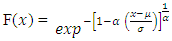 | (1) |
Its probability density function (PDF) is given as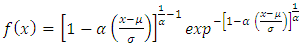 | (2) |
Where  is the scale parameter,
  is the shape parameter and
  is the location parameter. The value of
  dictates the tail behaviour of CDF. When
  is the Gumbel distribution, when
  is the Fréchet and when
 is the Weibull distribution.
2.1.1. Maximum Likelihood Estimation
If the set  are independent and identically distributed for a GEV distribution, then the likelihood and the log-likelihood function for a sample of n observations
  are given as follows;
  | (3) |
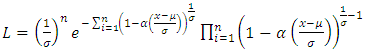 | (4) |
The log-likelihood function is given by | (5) |
The ML method requires the computation of the first-order partial derivatives of the log-likelihood function with respect to each of its parameters, equating them to zero and then solving the resultant equations. This yields the system of equations presented as follows: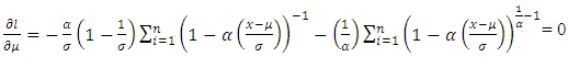 | (6) |
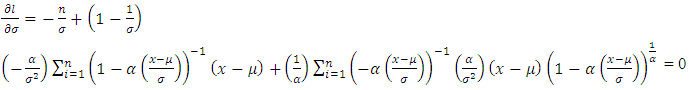 | (7) |
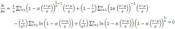 | (8) |
As there is no analytical solution for obtaining the maximum likelihood estimates of the GEV parameters, then, the three systems of the log likelihood equations will be solved by numerical means to obtain the parameters 
2.1.2. L-moments Estimation Method
Let  be a random sample of size r and let
  denote the corresponding order statistics. The rth L-moment defined by (Hosking 1990) as:
 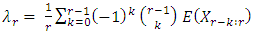 | (9) |
and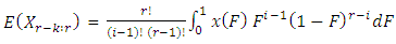 | (10) |
Therefore  | (11) |
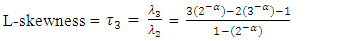
Where  and F are quantile function and cumulative distribution, respectively. The first four (Population) L-moment ratio were then defined by putting r = 1,2,3 and 4 is
 | (12) |
 | (13) |
 | (14) |
 | (15) |
The coefficients of the variation, skewness and kurtosis of the probability density function are 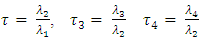 The sample L-moments are estimated from the sample order statistics which are defined by
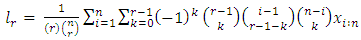 | (16) |
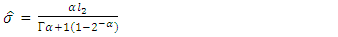
the equations can be obtained by equating the first three population L-moments to the corresponding first three sample L-moments, i.e., 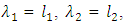 and
and  . Substituting the values of the population L-moments
  and
and  for the sample L-moments, The L-moments estimator of the parameters of the GEV distribution are given by
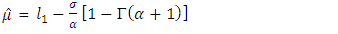 | (17) |
 | (18) |
 | (19) |
 | (20) |
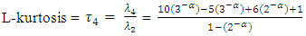
The shape parameter of the GEV will be estimated by using some approximation discussed by Hosking and Wallis (2005) i.e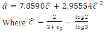 | (21) |
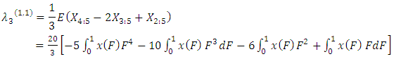
2.1.3. TL- Moment Estimators
Elamir and Seheults (2003) developedTrimmed L-moments (TL-moments) as generalisation of L-moments, in which they trimmed one smallest and one largest value from the conceptual sample. They proposed a more robust version of equation (10), in which E(X (r-k:r)) was replaced by 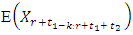 for each r where
  is the smallest and
  largest are trimmed from the conceptual sample. Theydenote this as
 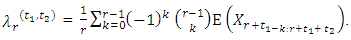 | (22) |
If the level of trimming becomes zero (i.e.,  ) the TL- moments reduce to L-moments. TL-moments in terms quantile function can be written as;
 | (23) |
The sample TL moment is given by | (24) |
In this work, we focused on trimming of  and the symmetric cases where
  .The first four TL-moments (1,0) can be written as follow
 | (25) |
 | (26) |
 | (27) |
 | (28) |
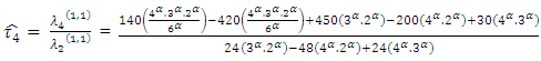
The TL- moment (1,0) estimators of the parameters of the GEV distribution are given by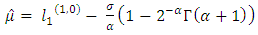 | (29) |
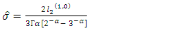 | (30) |
 | (31) |
Where  and
and  are the coefficients of the variation, skewness and kurtosisAlso, the first four TL-moments (1,1) can be written as follow
 | (32) |
 | (33) |
 | (34) |
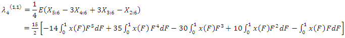 | (35) |
The sample TL-moment (1,1) can also be estimated by setting  in equation (24) aboveThe TL- moments (1,1) estimators of the parameters of the GEV distribution are given by
 | (36) |
 | (37) |
 | (38) |
 | (39) |
Where  and
and  are the coefficients of the variation, skewness and kurtosis.
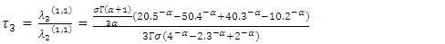
3. Method of Selection
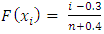
Mean square error (MSE) was used to select the best performing estimation methods considered in this work, it can be calculated as below. 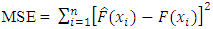 where
where  is the theoretical CDF at
 The results of estimates and MSE are presented in Table 1. The calculation was performed using computer programming language R and R studio.
3.1. Return Level and Return Period
The return period which is also known as recurrence interval, is an estimation of the likelihood of an event, such as rainfall, flood to occur. The return period (T) is expressed as  where
where  represents the probability of exceedance.Return levels for 5, 15, 45, 65, 85, and 105 return periods are estimated in this study. Inverting the GEV cumulative distribution, the return level is given by
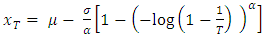
4. Presentation of Results
Table 1. Comparison of GEV parameters
 |
| |
|
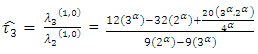
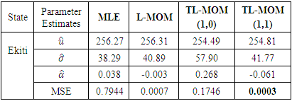
Interpretation: Table 1 shows the parameter estimation of GEV by the MLE, L-moment, TL-moments, using Ekiti state rainfall data. The results show that TL-moment (1,1) gave the least mean square error (MSE) value, which indicates that it is the most efficient estimator and it outperforms all the othermethods.Table 2. Prediction of Return Levels for Different Return periods in Ekiti State
 |
| |
|
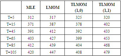
Interpretation: Table 2. also shows that the return level estimate by different methods of estimation increases as the return period increases. It was observed that the predicted return level estimates do not exceedmaximum rainfall amount of observation when T=5, T= 15. | Figure 1. Multiple Bar Chart showing return level for different return periods in Ekiti State |
Interpretation: Figure 1 presents return level of Ekiti State rainfall data using four estimation techniques.Table 3. Parameter Estimates of GEV by several methods Using Ondo Rainfall Data
 |
| |
|
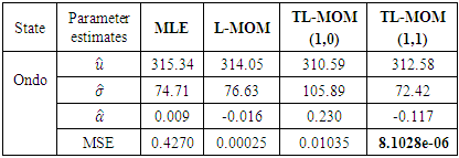
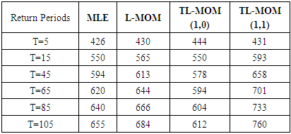
Interpretation: Table 3. shows the parameter estimation of GEV by the MLE, L-moment, TL-moments (1,0) and TL-moments (1,1) using Ondo state rainfall data. The results show that TL-moment (1,1) gave the least mean square error (MSE) value, which indicates that it is the most efficient estimator and it outperforms all the other three methods.Table 4. Prediction of return levels for different return period
 |
| |
|
Interpretation: The return level estimate increases as the return period increases. The point estimate of return level at T = 85, and even T = 105, exceed the maximum rainfall amount of the observation period.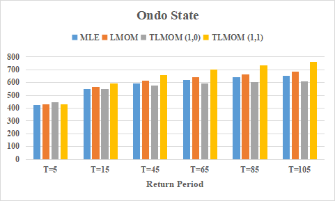 | Figure 2. Multiple Bar Chart showing rainfall recurrence interval for different return period in Ondo State |
Interpretation: Figure 2 presents return level of Ondo State rainfall data using four estimation techniques.
4.1. Discussion
Acomparative study of different estimation techniques for generalized extreme value distribution using rainfall data set oftwo different States in the Southwest, namely Ondo and Ekiti. The estimation techniques compared were the MLE, L-moments, TL-moments (1,0) and TL-moments(1,1). The mean square error estimate gives closely related results from one method to another. Considering the results in Table 1 and 3. it is obvious that the TL-moments (1,1) method outperformed other methods inEkiti and Ondo stations. The analysis in this study was further extended by estimating the prediction of return levels for T=5, 15,45,65,85 and 105 of return period. It was observed that the return level estimates increase as the return period increases in the two stations. Also, tables 1 and 4 showed the rainfall amount which exceeds the maximum rainfall amount of the observation period starts to appear at T = 45,65,85 and 105 it was observed that the best method in each station gave higher return periods.
5. Conclusions
In this work, we compared the performance of four different estimation methods for estimation of location, scale and shape parameters of generalized extreme value distribution. The estimates obtained from these methods are then compared using mean square error. The results show that the TL-moments (1,1) gave the least mean square error (MSE) value in Ekiti and Ondo. This indicates that TL-moments (1,1) is the most efficient estimator in the two selected states in southwestern zone of Nigeria considered in this work, while the MLE is the least efficient estimator with the highest mean square error. Also, the estimation of return level by different methods increases as the return period increases.
References
| [1] | Elamir E.A., Seheult A.H., (2003). Trimmed L-Moments, Computational Statistics & Data Analysis, 43(3), 299-314. |
| [2] | Gamage W., Hewa G.A., Subhashini W.H.C., Daniell T.M., and Kemp D., (2009). Modelling the extreme floods of South Australian catchments, MODSIM, 3435. |
| [3] | Hosking J.R., and Wallis J.R (1997) Regional frequency analysis: an approach based on L-moments. Cambridge University press. Cambridge. |
| [4] | Hosking J.R., (1990). L-Moments: Analysis and Estimation of Distribution Using Linear Combinations of Order Statistics. Journal of Royal Statistical Society. (B) 52: 105-124. |
| [5] | Hosking J. R., Wallis J. R., and Wood E. F., (1985). Estimation of the generalized extreme- value distribution by the method of probability-weighted moments. Technometrics, 27(3), 251-261. |
| [6] | Jenkinson, A. F., (1955). The frequency distribution of the annual maximum (or minimum) values of meteorological elements, Q. J. R. Meteorol. Soc., 81, 158–171. |
| [7] | Nadarajah, S. and Shiau, J.T. (2005). Analysis of extreme flood events for the pachang river, taiwan. Water resources management, 19(4): 363–374. |
| [8] | Park, J.S., Kang, H.S., Lee, Y.S. and Kim, M.K., (2010). Changes in the extreme rainfall in South Korea. International Journal of Climatology 31, 2290–2299. https://doi.org/10.1002/joc.2236. |
| [9] | Ramos, P. L., Louzada, F., Ramos, E. and Dey, S., (2020). Frechet Distribution: estimation and application an overview,” Journal of Statistics & Management Systems, vol. 23, no. 3, pp. 549–578. |
| [10] | Shabri A., (2002). Comparisons of the LH Moments and the L Moments, Matematika, 18, 33, |
| [11] | Wilks D.S., (2006). Continuous Distributions. In R. Dmowska, D. Hartmann, & H. Rossby (Eds.). Statistical Methods in the Atmospheric Sciences. Elsevier Inc. New York. Pp97. |
| [12] | Zalina, M.D., Desa, M.N.M. and Nguyen, V.T.A and Kassim, A.H.M. (2002). Selecting a probability distribution for extreme rainfall series in Malaysia, Water science and technology, Vol. 45, No. 2, 63–68. |
| [13] | Zin, W. Z. and Jemain, A. A. (2010). Theoretical and Applied Climatology 102(3), 253–264. |

 Abstract
 Reference
 Full-Text PDF
 Full-text HTML