Muhammad Alamgir Islam, Md. Shahidul Hoque, Maruf Hossain Afridi
Department of Statistics, University of Chittagong, Chattogram, Bangladesh
Correspondence to: Muhammad Alamgir Islam, Department of Statistics, University of Chittagong, Chattogram, Bangladesh.
| Email: |  |
Copyright © 2024 The Author(s). Published by Scientific & Academic Publishing.
This work is licensed under the Creative Commons Attribution International License (CC BY).
http://creativecommons.org/licenses/by/4.0/

Abstract
The economic growth of Bangladesh has gained significant attention in recent years. This study presents a comprehensive and in-depth exploration of forecasting the Gross Domestic Product (GDP) of Bangladesh using the Autoregressive Integrated Moving Average (ARIMA) model. The study precisely explores the ARIMA model, a widely familiar and powerful tool in time series analysis, and its application to the context of Bangladesh's GDP. In this research, data has been collected for the real GDP of Bangladesh from year 1960 to 2022 annually. The data is collected from the database of the World Bank and Kaggle Website. GDP Growth rates are also calculated annually. The autocorrelation function (ACF) and partial autocorrelation function (PACF) plot suggested a moving average of order one MA (1). The ARIMA models were obtained using the minimum Akaike Information Criterion (AIC) and Bayesian Information Criterion (BIC). Model diagnostics tests were performed using the Ljung-Box test and Augmented Dicky- Fuller (ADF) test. It is found that ARIMA (0, 2, 1) is the best model for forecasting the GDP of Bangladesh data series. Statistical outcomes illustrate that Bangladesh’s GDP will increase from 2023 to 2042. The results and insights from this study will help policymakers, stakeholders, and academics in economics to formulate business strategies more precisely.
Keywords:
ARIMA, Forecasting, GDP, Auto correlations, Stationarity, Time series, ADF Test
Cite this paper: Muhammad Alamgir Islam, Md. Shahidul Hoque, Maruf Hossain Afridi, Forecast Analysis of Bangladesh GDP on Economic Growth Using ARIMA Model, International Journal of Statistics and Applications, Vol. 14 No. 2, 2024, pp. 13-21. doi: 10.5923/j.statistics.20241402.01.
1. Introduction
Bangladesh has a strong track record of growth and development even in times of heightened global uncertainty. Bangladesh reached lower-middle income status in 2015. It is on track to graduate from the United Nations (UN) Least Developed Countries (LDC) list in 2026. A country's gross domestic product (GDP) is the monetary value of all final goods and services produced in a year by all enterprises within a country's borders. It presents aggregate statistics of all economic activities. Bangladesh’s GDP has been developing at a rapid pace in recent years. GDP is one of the significant indicators of national financial activity for the country. It provides a crucial assessment of a nation's economic health, growth trajectory, and overall economic activity. Systematic forecasting of indicators is the important theoretical and practical significance of the development of economic growth targets. It also becomes the root of understanding the nature and direction of the relationship between a country and its economic development process. It can be very helpful in formulating new policies and programs related to economic policy prepare the budget. Bangladesh's economy has suffered multiple shocks. Unnecessary from Russia's war in Ukraine and global monetary tightening have interrupted a strong post-pandemic recovery, with real GDP growth slowing to 6 percent in Fiscal Year (FY) 23 and headline inflation reaching a decade high of 9.9 percent year-on-year in August 2023.According to the provisional data of Bangladesh Bureau of Statistics (BBS), the GDP of Bangladesh is Tk. 44, 39,273 crore (US$ 454 Billion) in FY 2022-23, up by 11.77 percent from the previous FY. The per capita GDP increased to Tk. 2,59,919 in FY 2022-23. Time series analysis is a suitable method for making policy decisions, especially in health care, finance, business, and economics. GDP plays an important role in all economies as it helps the government formulate budgets and allows government agencies to make forecasts that help in the study of the growing economy as well as economic performance [1]. A significant change in GDP, up or down, usually affects a market economy. Therefore, it is necessary to understand the related factors affecting GDP. This is a reliable requirement for estimates of GDP over some future period, which is only possible by forecasting GDP as accurately as possible using an appropriate time series model.
1.1. Gross Domestic Product (GDP)
GDP is the total monetary or market value of all finished goods and services produced within a country's borders during a given period. As a broad measure of gross domestic product, it serves as a comprehensive scorecard of a given country's economic health. Although GDP is usually calculated on an annual basis, it is also sometimes calculated quarterly. The calculation of a country's GDP includes all private and government consumption, government spending, investment, additions to private inventories, paid construction expenditures, and the foreign balance of trade. Export value is added and import value is subtracted. Of all the components that make up a country's GDP, the foreign balance of trade is particularly important. A country's GDP increases when the total value of goods and services sold by domestic producers to foreign countries exceeds the total value of foreign goods and services purchased by domestic consumers. When this situation occurs, a country is said to have a trade surplus.
1.2. Literature Review
The amount of research done so far on GDP in Bangladesh is not enough to know the economy of the country. Hence, it is essential to forecast GDP for the estimated future economy as well as the progress of a country based on recent data. K. M. Salah Uddin et.al (2021) [2] found that the ARIMA (1, 2, 1) model is best appropriate for forecasting. Q-Q plot, residuals plot, PACF, and ACF graphs of the residuals are drawn to check model adequacy. They observed that the GDP trend has been steadily improving over the years in Bangladesh and will continue expanding in the forthcoming. Miah et al. (2019) [4] forecasted the GDP of Bangladesh and using model selection criteria and checking model adequacy and based on the ACF and PACF a time series model ARIMA (1, 2, 1) was chosen. It is observed that the values of GDP forecast in Bangladesh are gradually increasing over the next thirty years. Biplab Biswas et.al (2017) [7] Modelling and forecasting GDP at current market price in Bangladesh: an application of ARIMA model. ARIMA (0, 2, 1) model has been selected and it has been used to forecast GDP at the current market price of Bangladesh up to 2026-27. M. S. Azad et al. (2011) [13] used the ARIMA model in forecasting the Exchange Rates of Bangladesh. By using Box Jenkins methodology, they tried to find out best model for forecasting. They have found that the ERNN (exchange rate neural network) model shows better performance than ARIMA. The study by Bhattacharya et al. (2019) [3] used the data during a period from 1980-1981 to 2016-2017 to represent the forecasted value of the GDP of India for the year 2017-2018. They used a principal component augmented Time-Varying Parameter Regression (TVPR) approach and projected the model using a mix of fiscal, economic, trade, and creation side-specific variables. L. C. Voumik et.al (2019) [5] applied several ARIMA (P, I, Q) models and found that the ARIMA (1, 1, 1) model is best for forecasting. Also used Exponential Smoothing measurements to forecast the GDP growth rate. They have found the triple exponential model better analyzed the data based on the lowest Sum of Square Error (SSE) and Root Mean Square Error (RMSE). T. Liu et al. (2018) [6] Their study focused macroeconomic predicting model and proved the impact of the two-step technique. A simple single linear equation method is used here. To predict, an intuitive approach is to place all explanatory variables into the model equally. Wabomba et al. (2016) [8] identified the ARIMA (2, 2, 2) model as the best model for forecasting the Kenyan GDP. Their results indicated that the predicting effect of this model was relatively satisfactory and practiced in modeling the annual Kenyan GDP. Kumar et al. (2004) [15] used ARIMA model to forecast daily maximum surface ozone concentrations in Brunei Darussalam. They have found that ARIMA (1, 0, 1) was suitable for the surface O3 data collected at the airport in Brunei Darussalam. Liv et al. (2011) [11] used ARIMA model in forecasting incidence of haemorrhagic fever with renal syndrome in China. The goodness of fit test of the optimum ARIMA (0, 3, 1) model showed nonsignificant autocorrelation in the residuals of the model. Datta. K (2011) [14] used ARIMA model in forecasting inflation in the Bangladesh Economy. He showed that ARIMA (1, 0, 1) model fits the inflation data of Bangladesh satisfactorily. Al-Zeaud (2011) [12] used ARIMA model in modelling & forecasting volatility. The result shows that best ARIMA models at 95% confidence interval for banks sector is ARIMA (2, 0, 2) model. Uko et al. (2012) [10] examined the relative predictive power of ARIMA, VAR & ECM models in forecasting inflation in Nigeria. The result shows that ARIMA is a good predictor of inflation in Nigeria & serves as a benchmark model in inflation forecasting. J.C. Paul et.al (2013) [9] Selection of Best ARIMA Model for Forecasting Average Daily Share Price Index of Pharmaceutical Companies in Bangladesh: A Case Study on Square Pharmaceutical Ltd. They found that ARIMA (2, 1, 2) is the best model for forecasting the SPL data series. Contreras et al. (2003) [16] used ARIMA models to predict next-day electricity prices; they found two ARIMA models to predict hourly prices in the electricity markets of Spain & California. The Spanish model needs 5 hours to predict future prices as opposed to the 2 hours needed by the Californian model.This is clear from the above discussion many of the studies were done to forecast some economic variables using time series models but Bangladesh now needs to study GDP. In very few of them, the authors tried to find out the best ARIMA model, but in most of the articles, the authors used ARIMA to forecast. This report has attempted to identify the factors affecting the GDP forecast and the GDP of Bangladesh. The important objective of the study is to select the best ARIMA model and use this model in the GDP forecast of Bangladesh.
2. Data and Methodology
The data used in this paper are yearly Gross Domestic Product (GDP) from 1960 to 2022 obtained from the World Bank and Kaggle. Data consisting of 63 observations. The data to be used in this study is reliable because all sources of data are well-known, standard, widely used, and accepted by the government and others. A time series analysis method is used to analyze the real GDP data. For selecting the appropriate ARIMA model we have used AIC and BIC criteria. For predicting the GDP of Bangladesh from 2023 to 2042, the ARIMA model is used for forecasting.
2.1. Time Series Analysis
Time series analysis involves the systematic study of data collected or recorded in sequential order over a period. The primary goal is to understand patterns, trends, and underlying structures within the data to make informed predictions and decisions for the future.Autoregressive Integrated Moving Average (ARIMA)ARIMA is a widely used time series forecasting model known for its effectiveness and versatility. ARIMA combines autoregressive (AR), differencing (I), and moving average (MA) components to model sequential data. AR Component:The autoregressive component involves predicting a value in the time series based on its past values. It assumes that past observations have a direct influence on the current value. The order of this autoregressive term, denoted as "p," represents the number of past observations considered in the model.Mathematically, an AR(p) model is represented as Where ϕ1 is known as the first-order autoregressive coefficient, ϕ2 is known as the second-order autoregressive coefficient, and so on.Differencing (I) Component:Differencing involves taking the difference between an observation and a lagged observation (i.e., subtracting the previous value from the current value). This step aims to make the time series stationary, removing trends or seasonal effects. The differencing order, denoted as "d," signifies how many differences are needed to achieve stationarity.MA Component:The moving average component implies modelling the error term as a linear combination of error terms from previous time points. It captures the relationship between an error term at the current time point and error terms at previous time points.Mathematically, an MA(q) model is represented as
 Then we say that Y follows a qth order moving average or MA (q) process. In short, a moving average process is simply a linear combination of white noise error terms.The ARIMA model is denoted as ARIMA (p, d, q), where, p represents the order of the AR component d represents the order of differencing needed to achieve stationery and q represents the order of the MA component.The ARIMA (p, d, q) model can be mathematically expressed as
2.2. Model Selection Criteria
The Akaike Information Criterion (AIC) and Bayesian Information Criterion (BIC) are widely used model selection criteria to choose the best-fitting ARIMA model. They balance the model's goodness of fit with the complexity of the model. In the context of ARIMA modelling, lower AIC and BIC values indicate a better model fit.Akaike Information Criterion (AIC)AIC is an important and leading statistic by which we can determine the order of an autoregressive (AR) model. Mr. Akaike (1973) developed these statistics. According to his name, this statistic is known as the Akaike Information Criterion (AIC). AIC due to Akaike is defined as Where RSS= Residual sum of a square, p= number of parameters in the model, and n= sample size. The models with smaller AIC are preferred.Bayesian Information Criterion (BIC)Several modifications of AIC have been suggested. One popular variation called Bayes Information Criteria, originally proposed by Schwartz (1978), is defined as
  A lower BIC value indicates a better model.When selecting the appropriate ARIMA model using AIC and BIC, we would estimate multiple models with different orders (p, d, q) and choose the order that minimizes either the AIC or BIC.
2.3. Tests that are Used in This Study
Augmented Dickey-Fuller (ADF) TestIn the realm of time series analysis, the ADF test stands as a fundamental tool used to ascertain the stationarity of a time series. Stationarity is a crucial assumption for many time series models, including the Autoregressive Integrated Moving average. The ADF test serves as a hypothesis test to determine whether a given time series is stationary or non-stationary. It builds upon the original Dickey-Fuller test by including lagged differences in the series.Box TestIn time series analysis, the Box Test serves as a vital statistical tool for examining the presence of autocorrelation in data. Autocorrelation, or the correlation of a series with its past values, is a fundamental concept in time series analysis, influencing various modelling and forecasting techniques. The Box Test, often associated with the Ljung-Box test, assesses whether the autocorrelations of a time series up to a certain lag are significantly different from zero.
2.4. Plots that are Used in This Study
Autocorrelation Function (ACF):The ACF plot is a vital tool in time series analysis, showing the correlation of a time series with its lagged values. It visually presents how each observation is correlated with its previous observations at various lags. ACF plot helps to check the stationarity of the time series data.Partial Autocorrelation Function (PACF) The PACF plot is a crucial tool in time series analysis, offering insights into the direct relationship between a time series and its lagged values, removing the indirect effects of the intermediate lags. Each point on the PACF plot represents the correlation at a specific lag after removing the effects of intervening lags. Understanding the PACF plot is vital as it helps in model selection, especially when determining the order of the autoregressive component in a time series model. PACF plot also helps to check the stationarity of the time series data.
2.5. Proposed Model
To forecast GDP growth, the ARIMA model has been taken into consideration in this work.The proposed ARIMA (p, d, q) model can be mathematically expressed as where:Yt the time series at time t.L is the lag operator (i.e., LkYt=Yt−k).ϕ1, ϕ2,…,ϕp are the autoregressive parameters.θ1, θ2, …. θq are the moving average parameters.d is the degree of differencing needed to make the time series stationary.p is the order of the AR process.q is the order of MA process.εt is the error term at time t.
3. Data Analysis and Results Discussion
To forecast GDP growth, data on this macroeconomic variable was collected from 1960 to 2022 from the World Bank and Kaggle. It is a single set of data for modeling that was comprised of annual levels of GDP of Bangladesh in billion-dollar USD. The data file consists of 63 observations.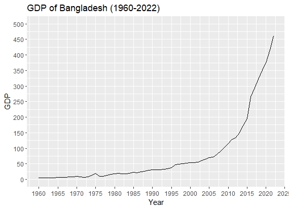 | Figure 1. GDP of Bangladesh in billion, USD (1960-2022) |
From the figure 1, we can see that the GDP of Bangladesh follows an upward trend. This shows that both the mean and the variance of the data are not stable. An upward trend in a time series plot of GDP typically signifies a consistent and sustained increase in the GDP values over time. This suggests that the economy is experiencing growth and expansion, at least during the observed period. Understanding and interpreting an upward trend in the GDP time series is essential for economic analysis and policymaking. Since we observe that the mean and the variance of the data are not constant, we can assume that the original data is non-stationary. Thus, we cannot apply the ARIMA model directly.
3.1. Autocorrelation and Stationarity Test
ACF plot of the GDP of Bangladesh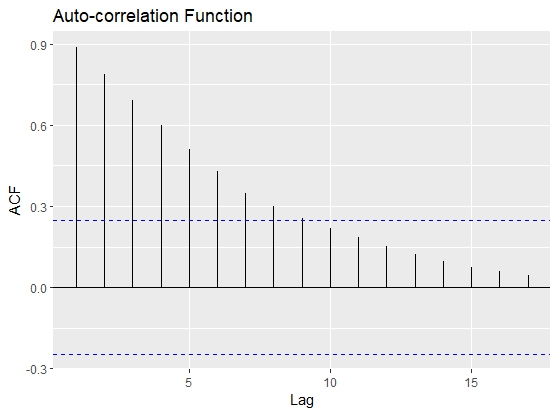 | Figure 2. Acf plot of the GDP of Bangladesh(1960-2022) (level data) |
PACF plot of the GDP of Bangladesh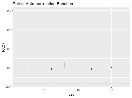 | Figure 3. PACF of GDP (Level data) |
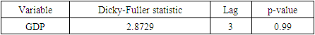
The Augmented Dickey-Fuller (ADF) test:H0: The time series is non-stationaryH1: The time series is stationaryTable 1. Results of the ADF Test on GDP Growth (original)
 |
| |
|
ACF plot after taking the second difference: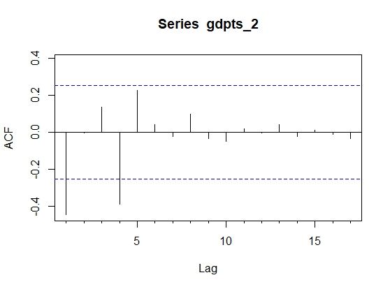 | Figure 4. ACF plot of the GDP of Bangladesh after taking the second difference |
PACF plot after taking the second difference: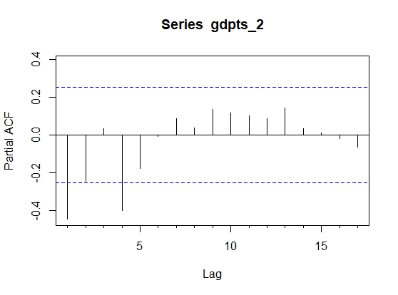 | Figure 5. PACF plot after the second difference |
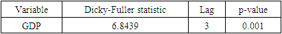
Table 2. Results of the ADF Test on GDP Growth (after second difference)
 |
| |
|
From Figure 2, we observe a gradual decline in the ACF of the GDP data indicating high autocorrelation between current and lagged values. This helps in identifying the pattern and dependencies in the data. The prominent peaks in the ACF plot indicate strong autocorrelation between the observations and their lagged values. The slow decay of the autocorrelation in the data as the lag increases demonstrates a gradual decline. Understanding these features in the ACF plot helps in choosing the appropriate lag values for building an ARIMA model.As we can see from the figure-3, there is a spike at lag 1. Other than that, the PACF plot does not pose much of a problem. Now, from Figure 2 and Figure 3, ACF and PACF of the original GDP series, we can say that the data is auto-correlated and also it is non-stationary. Now, we conduct the ADF test on the data to affirm the non-stationarity. The result in Table-1 confirms that GDP series follow a non-stationary pattern, which helps us to specify the Integrated (I) term in the ARIMA model. Since we have established that the data is non-stationary, we will take the first difference and again check for non-stationary by using the ACF plot, PACF plot, and ADF test. We observed that the original data is non-stationarity but after taking the second difference and checking by using the same plot and same test the time series data become stationary shown in Figures 4 & 5 and table-2.
3.2. Model Fitting
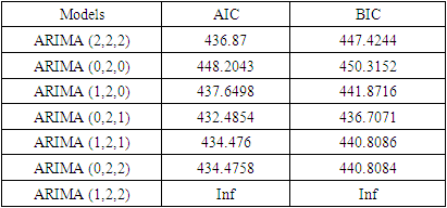
Now we fit the data with different ARIMA models to figure out the best ARIMA model as fitting the ARIMA model is an iterative process.Table 3. Different ARIMA models
 |
| |
|
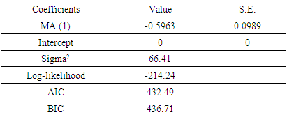
Since the AIC and BIC values are lowest for the AIRMA (0, 2, 1) model, it is the best-fitted model.The model summary:Table 4. Model summary of the best-fitted model
 |
| |
|
So, the fitted ARIMA (0, 2, 1) model can be written as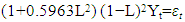
4. Major Findings of the Study
The principal findings of the study are as follows:The upward trends of plots of the data series are visualized although the overall trends are not smooth. The ACF and PACF plots of the original data series show that the GDP of Bangladesh is non-stationary, that is, most of the ACF and PACF plots are beyond the confidence limits (please see Figures- 2 & 3). From ACF and PACF plots of the data series taking first difference has been found that the GDP of Bangladesh data series is still non-stationary, that is, all the ACF & PACF plots are out of the confidence limits. But after taking the second difference of data series, the same plots show that the data is stationary (please see Figures 4 & 5). The Dickey-Fuller unit root test statistic also indicates that the GDP of Bangladesh data series is stationary. The computed absolute values of the  -statistic for GDP are found as
  = 2.8729, none of which exceeds the DF or Mackinnon DF absolute critical
  values (to be noted that 1%, 5%, and 10% level of significance in the absolute DF values are 4.047, 3.462 & 3.13 respectively) (please see the Table-1). After taking the second difference of the GDP of Bangladesh data series, the same test statistic shows that the data is stationary because hence the computed absolute value of the
  -statistic is
  = 6.8439 which exceeds the DF or Mackinnon DF absolute critical
  values (please see the Table-3). For the GDP data series ten types of tentatively ARIMA models with varied values of p, d & q are selected of which seven-performed models for the data series are estimated as shown in Table -3. It is found that ARIMA (0, 2, 1) is the best model for forecasting the GDP of Bangladesh data series. Finally, the GDP of Bangladesh data series has been forecasted by using the selected model and reported in Table 5.
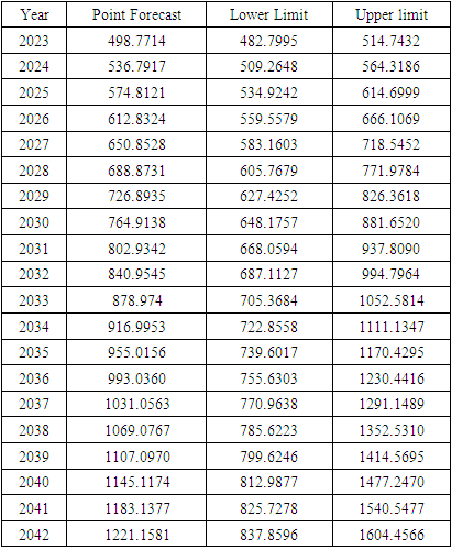
5. Forecasting GDP for Bangladesh
Table 5. Forecasted values for GDP prices (Billions of U.S dollars)
 |
| |
|
Plot of the forecasted GDP of Bangladesh: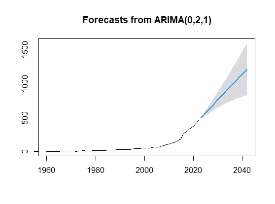 | Figure 6. Plot of the forecasted GPD |
5.1. Autocorrelation Test of the Forecasted GDP
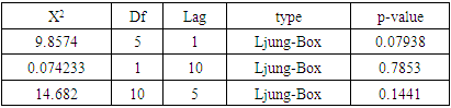
Ljung-Box test:Hypothesis: H0: There is autocorrelation.H1: There is no autocorrelation.Table 6. Test results
 |
| |
|
Since the p-value of the test is more than 0.05 for different lags, we can conclude that there is no auto-correlation in the forecasted GDP data.
6. Conclusions and Implication
This study attempted to establish an appropriate ARIMA model to describe the time series data using the ADF test and Ljung Box Q statistic. For this purpose, time series data on annual GDP from the period were 1960 to 2022 examined as the sample time series data. The time series data set included a total of 63 annual observations. Primarily the data series was found non-stationary. The ACF and PACF plot shows the original data series is non-stationary and after taking the second difference same test and plot show that the data series become stationary. Going through the process of identification and estimation, several ARIMA (p, d, q) models were estimated. Diagnostic checking on all estimated models was conducted based on AIC and BIC criteria for selecting the best-fitted model. The results of the diagnostic check established the ARIMA (0, 2, 1) model as the most efficient model. The GDP of Bangladesh is forecasted by using the model. From the predicted values, Bangladesh's GDP shows a higher growth trend in the years 2023 to 2042. Bangladesh will progress its position from under developing country to a developing country with appropriate forecasted time.The findings of this study have some important implications for academicians, policymakers, finance authorities, and researchers. Also, this study will encourage them to conduct further studies about forecasting GDP growth in Bangladesh. The findings will be better if future researchers take into consideration the other models such as the State Space model, Markov Switching model, Vector Autoregressive (VAR) model, and Vector Error Correction Model (VECM).
Limitations
The study is based on secondary data. Thus, limitations of secondary data remain in the study. In this study, the model is established using the ARIMA method only. Other types of time series models such as ARCH, GARCH, and VAR models were not considered. A fundamental limitation of this study is the length of GDP data points used. Although the ARIMA modeling process can be applied if the length of data points exceeds 50 observations, it is still not sufficient. This study examines the movement of Bangladesh's total GDP to test the efficient ARIMA model. Bangladesh however has different sectoral components of GDP such as industry, agriculture, and service sector GDP. The movement of these components of GDP can follow different patterns, and therefore unique ARIMA models can be efficient in capturing the movement of each of these components of GDP. Therefore, future studies are recommended to examine efficient forecasting models for sectoral GDP. Moreover, this study was limited to selecting only the best-performing ARIMA model in capturing the GDP movements of Bangladesh.
References
| [1] | B. S. Borbor et.al (2022) Forecast Analysis of Ghana’s Gross Domestic Product in Economic Growth using Time Series ARIMA, Asian Research Journal of Mathematics 18(2): 47-55. |
| [2] | K. M. Salah Uddin et.al (2021), Forecasting GDP of Bangladesh Using ARIMA Model, International Journal of Business and Management; Vol. 16, No. 6. |
| [3] | Bhattacharyaa et al. (2019), Forecasting India’s economic growth: a time-varying parameter regression approach. Macroeconomics and Finance in Emerging Market Economies, 1-24. |
| [4] | Miah et.al (2019). Modelling and forecasting of GDP in Bangladesh: An ARIMA Approach. Journal of Mechanics of Continua and Mathematical Sciences, 14(3), 150-166. |
| [5] | L. C. Voumik et.al (2019) Forecasting GDP growth rates of Bangladesh: an empirical study, Indian Journal of Economics and Development, Vol 7 (7). |
| [6] | T. Liu et al. (2018) Forecasting Chinese GDP using online data. Emerging Markets Finance and Trade, 54(4), 733-746. |
| [7] | Biplab Biswas et.al (2017) Modelling and forecasting GDP at current market price in Bangladesh: an application of ARIMA model, International Journal of Advanced Research 5(2), 1223-1232. |
| [8] | Wabomba, M. S. et.al (2016). Modelling and forecasting Kenyan GDP using Autoregressive Integrated Moving Average (ARIMA) models. Science Journal of Applied Mathematics and Statistics, 4(2), 64-73. |
| [9] | J.C. Paul et.al (2013) Selection of Best ARIMA Model for Forecasting Average Daily Share Price Index of Pharmaceutical Companies in Bangladesh: A Case Study on Square Pharmaceutical Ltd., Global Journal of Management and Business Research Finance Volume 13 Issue 3 Version 1.0. |
| [10] | Uko, A.K; Nkoro, E. (2012) “Inflation Forecasts with ARIMA, Vector Autoregressive & Error Correction. |
| [11] | Liv, Q.; Liu, X.; Jiang, B. & Yang, W. (2011) “Forecasting incidence of haemorrhagic fever with renal syndrome in China using ARIMA model”, Biomed Central, pp. 1-7. |
| [12] | Al-Zeaud, H.A. (2011) “Modelling &Forecasting Volatility using ARIMA model”, European Journal of Economics, Finance & Administrative Science, Issue 35, pp. 109-125. |
| [13] | Azad, A.K. & Mahsin, M. (2011) “Forecasting Exchange Rates of Bangladesh using ANN & ARIMA models: A comparative study, International Journal of Advanced Engineering Science & Technologies, Vol. No. 10, Issue No. 1, pp. 031-036. |
| [14] | Datta, K. (2011) “ARIMA Forecasting of Inflation in the Bangladesh Economy”, The IUP Journal of Bank Management, Vol. X, No. 4, pp. 7-15. |
| [15] | Kumar, K.; Yadav, A.K.; Singh, M.P.; Hassan, H. and Jain, V.K. (2004) “Forecasting Daily Maximum Surface Ozone." |
| [16] | Contreras et.al (2003) “ARIMA models to predict Next Day Electricity Prices,” IEEE Transactions on the power system, Vol. 18, No. 3, pp 1014-1020. |

 Abstract
 Reference
 Full-Text PDF
 Full-text HTML