1. Introduction

It does not happen often that the results of a largely statistical study make it into the headlines of the major international news media. One example is the prediction of the imminent collapse of the Atlantic Meridional Overturning Circulation (AMOC) by Ditlevsen & Ditlevsen (2023). In view of the significance of such an event for the global climate, it is not surprising that their study has caused quite a stir. However, Reschenhofer (2023a) pointed out some of the weaknesses of this study. Indeed, it looks at first glance like voodoo statistics when the possible transition from the present strong AMOC mode to a weak AMOC mode is equated with the transition of some AMOC proxy from a stationary state with first-order autocorrelation ρ less than one to a nonstationary state with ρ=1. This magical connection results from the choice of a specific stochastic differential equation for the description of the dynamics of the AMOC proxy and the application of a set of more or less plausible assumptions and approximations (for an in-depth critical examination see Reschenhofer, 2023a). But even if there were no serious flaws in this approach, there would still be the difficult task of extrapolating the autocorrelation. The underlying dynamic model provides only the monotone transformation intended to make the increase in autocorrelation reasonably linear. The beginning of the rise in autocorrelation and the size of the rolling estimation window must be chosen in a more subjective manner. Ditlevsen & Ditlevsen (2023) accomplished this by trying out many different values, which clearly increases the risk of a data-snooping bias and impairs any subsequent inference. But that does not matter anyway in view of Reschenhofer’s (2023a) finding that the autocorrelation increases erratically rather than steadily, which makes forecasting based on extrapolation basically impossible.

Apart from methodological issues, there are also data issues. Since direct measurements of the AMOC are only available for relatively short periods (Smeed et al., 2014), proxies for the strength of the AMOC must be used instead. Such a proxy is typically defined as the difference between the mean sea surface temperature (SST) in some northern sea region with below-average warming and some global or hemispheric benchmark. The most widely used region is the subpolar gyre (see Rahmstorf et al., 2015), which contains the 17 grid points represented by circles with black borders in Figure 1. Examples of benchmarks are the Northern Hemisphere mean surface temperature (Rahmstorf et al., 2015) and the global mean SST (Caesar et al., 2018). Ditlevsen and Ditlevsen (2023) used two times the global mean SST in order to compensate for polar amplification (see Holland and Bitz, 2003). However, Reschenhofer (2023a) argued that the subtraction of a benchmark may be counterproductive when the main task is to monitor early-warning signs like a rising autocorrelation. For the estimation of autocorrelation, the trend must be removed anyway, regardless of whether it is just the regional trend or the combined regional and global trend. So all that remains is the noise. But why would anyone want to pollute the interesting regional measurements with global noise or even two times global noise?

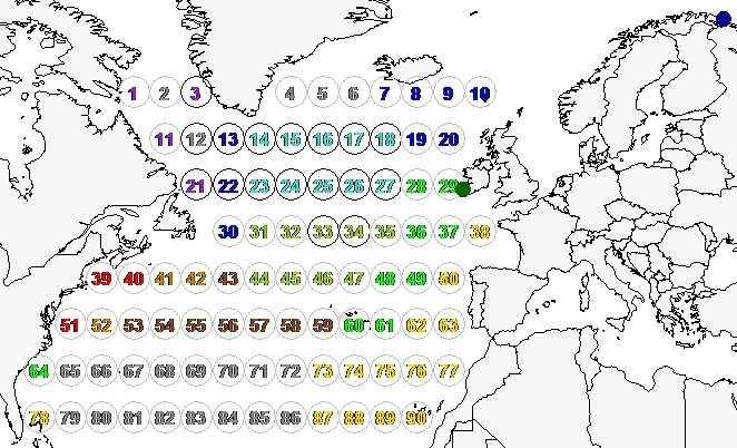Figure 1. Nine clusters (purple, blue, turquoise, green, yellow green, yellow, red, orange, brown) of grid points and two stations (Valentia Observatory, Ireland: dark green, Vardo, Norway: dark blue)

Another factor of uncertainty is the definition of the sea region that is used for the construction of the AMOC proxy. Reschenhofer (2023b) identified a region in the north of the subpolar gyre which appears to be still defying global warming. However, a closer look revealed seasonal differences. Recently rising temperatures in the months from July to October suggest that global warming is finally catching up with this region. From a statistical point of view, this development creates two problems. Firstly, the emergence of any distinct trend will inevitably mask the Atlantic Multidecadal Oscillation (AMO), which contributes significantly to the autocorrelation because of its large amplitudes and long cycle lengths. In the course of a standard trend-removal procedure, the AMO will then be removed together with the trend and the estimated autocorrelation will therefore show a non-genuine decline. Secondly, any change in the seasonal pattern will inevitably distort the estimation of the autocorrelation if the seasonal adjustment is carried out in the usual naive way. Temperature measurements are typically expressed as anomalies from the base period 1961-1990 (CRU, University of East Anglia) or 1951-1980 (NASA GISS), where the average temperature for each calendar month in the base period is regarded as normal. Alternatively, the anomalies may be obtained by subtracting the monthly means over the full observation period. Clearly, either method is only appropriate in the case of a constant seasonal pattern.

In the next section, a more sophisticated procedure will be proposed which allows for the simultaneous removal of the trend and any constant or time-changing seasonal pattern. Afterwards, a graphical procedure will be presented in Section 3 which allows for the instantaneous and unbiased assessment of the size of the autocorrelation. Both procedures will be applied to monthly temperature series. The empirical results will be discussed with regard to the usefulness of the estimated autocorrelation as a potential early-warning sign. Section 4 concludes.

2. Seasonal Adjustment and Detrending

The dataset HadCRUT5 Analysis, which combines land [CRUTEM5] and marine [HadSST4] temperature anomalies from the base period 1961-1990 on a 5° by 5° grid with greater geographical coverage via statistical infilling (Morice et al., 2021), was downloaded from the website https://crudata.uea.ac.uk/cru/data/temperature/ of the Climatic Research Unit (CRU) of the University of East Anglia. Station data were downloaded from the website //data.giss.nasa.gov/gistemp/ of NASA's Goddard Institute for Space Studies (GISS). These are adjusted, cleaned data, homogenized to account for urban effects (GISTEMP Team, 2023; Lenssen et al., 2019). The common analysis period for both types of time series is from January 1880 to November 2023 (n=1727 months). For the statistical analysis, the free statistical software R (R Core Team, 2022) was used.

Figure 1 shows nine clusters of grid points with similar temperature trends according to Reschenhofer (2023b) as well as the meteorological stations Valentia Observatory (51.9394N, 10.2219W) and Vardo (70.3670N, 31.1000E). The main reason for the selection of these two stations was the availability of the data. There is only one missing value in the case of Valentia Observatory, namely in November 1942, which was replaced by the average of the values in October 1942, December 1942, November 1941, and November 1943, and also only one missing value in the case of Vardo, namely February 2023, which was replaced by the average of the values in January 2023, March 2023, and February 2022. In addition to the two stations, three grid points were selected for further analysis, namely 11, 16, and 29. The first represents the cluster with the most noticeable changes in the seasonal pattern (see Reschenhofer, 2023b), the second represents the northern part of the subpolar gyre, and the third is of interest because of its proximity to Valentia Observatory. The data from CRU are anomalies from the base period 1961-1990 whereas the data from GISS are absolute values. In the case of the anomalies, a seasonal pattern only becomes visible when it changes over time.

Let be any one of the five time series of anomalies or absolute values. For each calendar month, i.e., j=1,...,12, the trend of the subseries

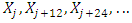(1)

can be estimated by smoothing with the Hodrick-Prescott (HP) filter (using the R function hpfilter of the package mFilter), i.e., by minimizing

(2)

where the tuning parameter Λ determines the degree of smoothing. The estimated monthly trends obtained with Λ=2.5∙10^3 and Λ=2.5∙10^4, respectively, are shown for each of the five time series in Figure 2. Strictly speaking, only the latter can be regarded as trend estimates. The more volatile trend lines obtained with the smaller value of Λ are only meant to make significant oscillations like the AMO visible. As the upward trend picks up speed, it might soon mask the AMO even in regions like the subpolar gyre and thereby make the monitoring of the autocorrelation pointless. For purely technical reasons, there can be no further increase under these conditions.

Figure 2. HP trends (Λ=2.5∙10^3) from January 1880 to November 2023 for each calendar month (January: purple, February: blue, March: turquoise, April: dark green, May: green, June: yellow green, July: red, August: pink, September: yellow, October: orange, November: brown, December: gray) as well as smoother HP trends (Λ=2.5∙10^4 , black) (a)-(c): Grid points 11, 16, and 29, (d): Valentia Obs., (e): Vardo

What is also striking in Figure 2 are the discrepancies between different calendar months, e.g., a strongly above-average temperature rise from January to March in the case of grid point 11 and a strongly above-average temperature drop from January to March in the case of grid point 16. In such a situation, the naive seasonal-adjustment method of just subtracting the monthly means is not appropriate. Figure 3 compares the naive method with the more sophisticated method which subtracts the monthly HP trends (Λ=2.5∙10^4). The first column of Figure 3 shows the downloaded data, which are in the case of the three grid points anomalies and have therefore already been adjusted by subtracting the monthly means over the base period 1961-1990. The time series in the second column were adjusted by subtracting the monthly means over the full observation period. They were plotted together with HP trends obtained with a much larger value of the tuning parameter, namely Λ=2.5∙10^9. This choice is due to the much higher frequency. In contrast to the monthly subseries (1), there are now 12 values per year instead of only one. In addition, HP trends with Λ=2.5∙10^7 were also included to illustrate the strength of the AMO. The time series in the third column were obtained by subtracting monthly HP trends (with Λ=2.5∙10^4). As was to be expected, there is no longer a trend here because this adjustment method removes the seasonal pattern and the trend simultaneously.

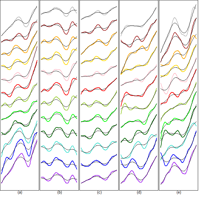
Figure 3. First column: Downloaded data (Jan. 1880 - Nov. 2023) Second column: Adjusted by subtracting monthly means (with fitted HP trends, Λ=2.5∙10^9 : yellow, Λ=2.5∙10^7 : magenta) Third column: Adjusted by subtracting monthly HP trends (Λ=2.5∙10^4) (with fitted HP trends, Λ=2.5∙10^9 : yellow, Λ=2.5∙10^7 : magenta) First 3 rows: Grid points 11, 16, 29. Last 2 rows: Valentia Obs., Vardo

Clearly, it depends on the respective type of analysis how serious the consequences of a botched seasonal adjustment are. The next concrete task we are facing is to look for indications of a rising variance or a rising first-order autocorrelation, which have both been used as early-warning signs for an AMOC collapse by Boers (2021) and Ditlevsen and Ditlevsen (2023). Figure 4 examines the extent to which the choice of the seasonal-adjustment method influences the estimation of the second moments. Three variants are considered, namely the two naive methods which simply subtract the monthly means over the base period 1961-1990 and the full observation period, respectively, and the more sophisticated method which subtracts the monthly HP trends (with Λ=2.5∙10^4). In the first two cases, the seasonally adjusted time series will still have a trend, which has to be removed with the help of another HP filter before second moments can be calculated. For this purpose, the value Λ=2.5∙10^9 was chosen. For the residuals remaining after seasonal adjustment and detrending, the statistics and were plotted cumulatively against time, where

(3)

and (Reschenhofer, 2017a, 2017b, 2019). These cumulative graphs allow the detection of any changes without the delay caused by a large estimation-window width of 50 (Ditlevsen and Ditlevsen, 2023) or even 70 years (Boers, 2021). Remarkably, the actual changes in the variance (shown in the first column of Figure 4) and the autocorrelation (in the second column) are easier to explain by structural breaks in the slope than by a steady growth of the slope, which corroborates earlier findings (Reschenhofer, 2023a, 2023b). Regarding the differences between the different adjustment methods, one would expect that any remaining part of the seasonal pattern will cause a rise both in variance and autocorrelation. Indeed, the variance appears to be consistently higher whenever a naive adjustment method is used. To a lesser extent, this is also true for the autocorrelation.

Figure 4. Cumulative estimation of variance (from Jan. 1880) left and cumulative estimation of autocorrelation (from Feb. 1880) right Adjustment methods: Subtracting monthly HP trends (blue) Subtracting monthly means over full observation period (green) Subtracting monthly means over the base period 1961-1990 (red) First 3 rows: Grid points 11, 16, 29. Last 2 rows: Valentia Obs., Vardo

The statistic is a severely biased estimator for the first-order autocorrelation ρ unless ρ is close to zero. However, when we are mainly interested whether ρ is rising or not, a possible bias does not matter that much. Nevertheless, an alternative, unbiased monitoring procedure will be used in the next section.

3. Estimation of Autocorrelation

Assuming that any trend or seasonal pattern has already been removed from the time series by subtracting monthly HP trends (as described in Section 2), the current variance and first-order autocovariance can easily be estimated by and respectively. In the case of the first-order autocorrelation, it is not that simple. The replacement of the highly unstable least squares estimator

(4)

by Burg’s estimator

(5)

(Burg, 1967, 1975) does bring a certain stabilization because the latter does not take values outside the open interval (-1,1) with positive probability, but there is still a large bias. Unfortunately, the same is true for the estimator (3), which has been designed for the monitoring of financial data under the assumption of a weak autocorrelation. In the case of temperature data, an assumption such as (see Reschenhofer, 2017a) is certainly highly implausible (see Figure 4). So, if we are also interested in the size of the autocorrelation and not just whether it goes up or down, we need an alternative method. For the determination of the direction alone it would be sufficient to plot the statistics (3) or (5) cumulatively against time. In contrast, plotting the statistics seems to be pointless at first glance because it is impossible to tell whether a rise in the auto-covariance is due to a rise in the variance or a rise in the autocorrelation. At second glance it is the solution. Indeed, plotting the statistics together with the statistics for various values of allows the unknown auto-correlation to be determined with sufficient accuracy for practical use. Alternatively, the differences can be plotted which often results in a clearer display. Both types of plots are shown in Figure 5. The autocorrelation is very weak in the case of the two stations and very high in the case of grid point 16 which lies in the subpolar gyre and can therefore possibly serve as an indicator for the strength of the AMOC. In the latter case, the cumulative differences 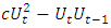are remarkably flat for c=0.7 (yellow line) until the early 1940s, for c=0.8 (green line) until the late 1990s, and finally slightly increasing for c=0.9 (blue line), indicating that the autocorrelation is first about 0.7, then about 0.8, and finally slightly below 0.9. In each period, the respective cumulative graph is roughly linear. Moreover, there is no indication of a smooth transition from one period to the next. The transitions rather look like structural breaks.

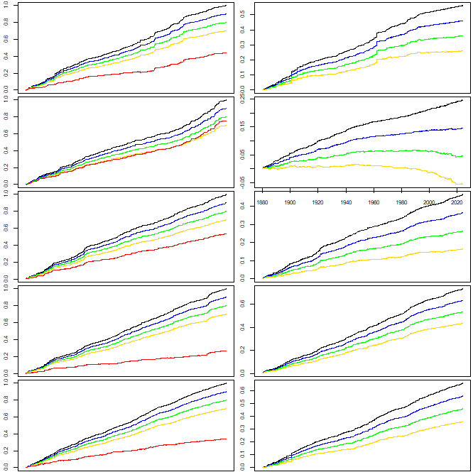Figure 5. Comparing the cumulative first-order autocovariance (red) from February 1880 to November 2023 with 1 (black), 0.9 (blue), 0.8 (green), and 0.7 (yellow) times the cumulative variance. The second column is obtained from the first by subtracting the red line from the other lines. First 3 rows: Grid points 11, 16, 29. Last 2 rows: Valentia Obs., Vardo

4. Discussion

The prediction of an imminent collapse of the AMOC (Ditlevsen and Ditlevsen, 2023) is based on a specific dynamic model for a specific AMOC proxy and on the assumption that the model parameter λ, which is related to the first-order autocorrelation ρ of the AMOC proxy via

(6)

grows linearly over time until it reaches a critical point where the dynamical system will move to a different state. While the model and the proxy have already been discussed at length in previous papers (Reschenhofer, 2023a, 2023b), the focus of the present paper is solely on the estimation of ρ, which is an important part of the prediction because the time of transition is found by extrapolating estimates of ρ up to the point where the value 1 is reached.

In light of evidence that global warming affects the different seasons differently, the standard method to remove seasonal patterns by simply subtracting monthly means is not suitable. Instead, HP smoothing is carried out separately for each calendar month, which allows to remove trends and seasonal patterns simultaneously just by subtracting the HP trends. This method saves the effort to keep time-changing trends and time-changing seasonal patterns cleanly apart.

After the removal of any trend and seasonal pattern, the time-changing autocorrelation of the residuals can be estimated. In order to avoid any delay caused by using a rolling estimation window, this is done by examining the slopes of the cumulative differences 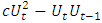for various values of c. The results obtained for the sea surface temperature in a region that is often used for the construction of AMOC proxies show that ρ is still smaller than 0.9 and there is no indication of a further increase toward 1. The method of predicting the time of a possible AMOC collapse by extrapolation therefore lacks any basis.