1. Introduction

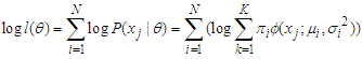
According to Lindsay (1995), Mixture Models (MM) as probabilistic models are used for representing the presence of population subsets located within an overall population. Mixture models provide a much wider range of modeling possibilities and capabilities than the single component model. Some details of MM can be found in Bohning and Seidel (2003) and Bohning et al. (2007).

For estimation involving mixture models, various analytical methods have been developed for estimating (a parameter space) in finite mixture models. There are many methods of estimating the parameters of a MM, four of such methods are method of moments, minimum distance method, Bayesian method and maximum likelihood (ML) method.

Pearson’s (1894) method of moments is one of the earliest methods for estimating the parameters from finite mixture models. This method held sway until the advent of modern computers to compute the maximum of the log-likelihood function. Some developments in the method of moment estimation can be found in Lindsay & Basak (1993), Furman & Lindsay (1994a, b), Lindsay (1995), Withers (1996) and Craigmile & Titherington (1998).

Minimum distance estimation methods introduced by Wolfowitz (1957) is a general method for estimating in a finite mixture, have been discussed by William et al. (1982) and Titherington et al. (1985).

Another method for estimating is the Bayesian method. Many reasons abound why some researchers are inclined to using Bayesian method of estimation while dealing with a finite MM (Fruhwirth-Schnatter, 2006). The reasons for these are the introduction of a suitable prior distribution or that eliminates spurious modes in the course of maximizing the log-likelihood function, and secondly, in the case where the posterior distribution for the unknown parameters is handy, this method provides reliable inference without recourse to the asymptotic normality of the distributions. These are the inherent advantages associated to this method especially when the sample size is small , since the asymptotic theory of MLE can be implemented when is quite large .

The fourth method for estimating the parameters of a finite MMs is the ML Estimation method. Likelihood based inference has enjoyed tremendous and fast developments and has contributed immensely towards resolving estimation problems involving finite MMs. Since the explicit expression for the MLE’s are typically unavailable, then a numerical EM Algorithm is used for maximizing the log-likelihood function. The expectation-Maximization (EM) Algorithm is one of the methods frequently in use according to Dempster et al. (1977). We can find more details about this methods in McLachlan and Krishna (1997), McLachlan and Peel (2000), Oleszak (2020), Kuroda (2021) and Smyth (2021).

The aim of this paper is to implement classification procedure on the Gaussian mixture model involving 2 groups and to identify the component from which each group elements probably belongs to, and as well as to estimate the respective parameters of the groups and their mixture weights. The EM Algorithm procedures were implemented in this paper using MATLAB.

2. Methods

Let be a random variable from a normal population. Let also be a random sample from that constitute two groups, such that

where .

According to Wirjanto (2009), we assume that 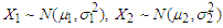. The Gaussian distribution is defined as

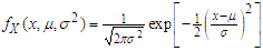(1)

, so that the probability density function of mixture of Gaussians will be given as

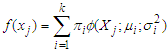(2)

where and are the mixing parameter weights.

In two component Gaussian mixture models, and is the PDF of a normal distribution with finite mean and finite variance . The number of estimable parameters of the Gaussian mixture distributions is given by the formula so that if , as in our case, .

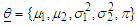2.1. Implementation Procedure of EM Algorithm

Dempster et al (1977) and Wu (1985) have proposed the use of initial guesses for the parameters Soderlind (2010) in line with Dempster et al (1977) and Wu (1985) suggested using Both and can be set equal to the overall sample variance Here, we take , similarly for . We initialize the mixing proportion at .

(a) e-step:

Following Huber (1964), for a given number of an observed data, we can evaluate the corresponding posterior probabilities, called responsibilities as follows

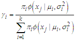(3)

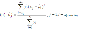
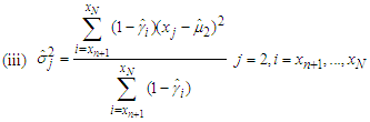
for and

(b) m-step:

Now, we compute the weighted means and variances using the obtained responsibilities in (3) as

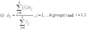(4)

(5)

(6)

The mixing probability is computed as;

(7)

Naturally, iteration continues until convergence is achieved. Convergence is generally achieved by evaluating the log-likelihood after performing each iteration and stop further iteration when it appears that the log-likelihood is not changing in a significant manner from one iterative step to another. In Kiefer & Wolfowitz (1956), under the independent and identically distributed (iid) assumption, the log-likelihood is defined as follows:

(8)

The up-dated mixture mean and variance are obtained if we have as a random variable with a two component Gaussian mixture as follows: Representing the mixture mean weight as and that of the mixture variance weight then the respective mixture mean and variance weights can be estimated respectively as

(9)

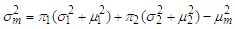(10)

where and is the up-dated mean and variance of the Gaussian mixture after each iterative step of the EM Algorithm.

2.2. Classification with Gaussians

We used Bayes’ Theorem for our problem to relate the probability density function of the data, , given the class to the posterior probability or the class given the data. Considering our univariate data consisting of a set of random variable , whose PDFs, given , are Gaussians with means and variances . Using Bayes’ theorem, we specify the component probability density function as;

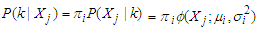(11)

where is the likelihood of class given observation . Probability of misclassification is a measure of the likelihood that individuals or objects are classified wrongly. We have two types of misclassification error as;

1. To classify into population given that it is actually from population

2. To classify into population given that it is actually from population

Following Richard et al. (2007), we classify the classification against the true group by creating a Statistician’s Confusion Matrix as in Table 1. Apparent error rate can be defined as the measure of performance in classification that does not depend on the form of the parent population. This rate is the fraction of observed values in the training sample that are misclassified by the sample classification function and can be calculated for any classification procedure. The confusion matrix is of the form

Table 1

where

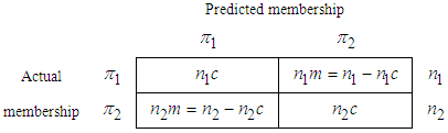
Number of objects that are correctly classified as objects

Number of objects misclassified as objects

Number of objects that are correctly classified into objects

Number of objects that are misclassified into objects.

The formula error rate is given as

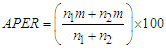(12)

See Appendix G for the MATLAB Source codes of obtaining the relevant quantities in Table 1.

3. Results and Discussions

Two data sets were used. Data Set 1are weights of male and female first year students of Abia State Polytechnic, Aba. Data Set 2 consists of weights of 120 males and 80 female babies at birth from Federal Medical Centre (FMC), Owerri, Imo State. See data on Appendix A, B and C. In this section, we used MATLAB source codes to implement the EM Algorithm procedures and as well, carry out the data classification analysis.

3.1. Result of the Expectation Step

Using Data set 1, taking initial values for . We also take the overall mean . is an column vector of the combined weights of male female students. We generate the probabilities for each of the data points. This step helps us in allocating the distinct mixture observations to previously defined groups. See equations (1) - (7) in page 3-4. Using Data set 2, the Algorithm was initialized with the following parameter values, , taking its overall initial mean as . In this case, is a column vector of the combined baby weights at birth. Data set 1 consist of while in Data set 2, since, and .

3.2. Results of the Maximization Step

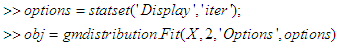
For us to obtain the log-likelihood and the mixing proportions using Data sets 1 & 2, we applied the MATLAB code in Appendix F. This approach, maximizes the E-Step and outputs the optimal mixing weights using data set 1 as ,and component means as 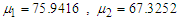& component variances as , . Using data set 2 in the same manner, we obtained the final requisite parameter up-dates as , , component means as 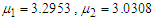, and component variances as 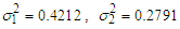. See equations (9) - (10) in page 4 of this paper.

3.3. Results of the EM Algorithm

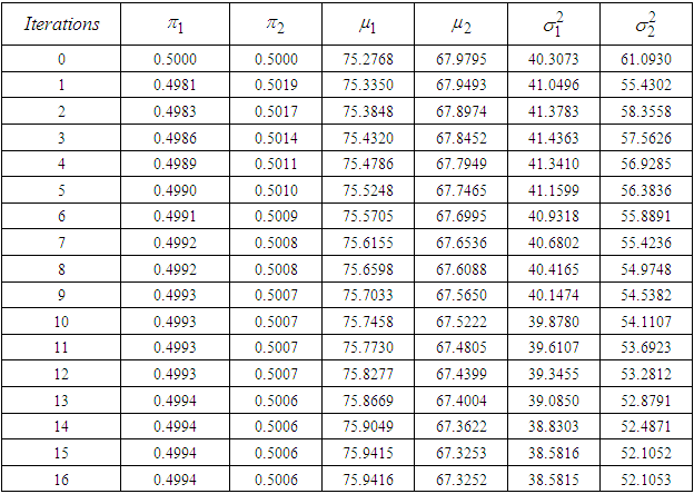
Data set 1

After our implementation of the EM algorithm using data set 1, the iterated maximum likelihood estimates for the parameters are contained in Table 2.

Table 2. Results of estimation of model parameters using data set 1

To achieve convergence, 17 iterations were required for optimality criterion, with log-likelihood = -3492.46. See source codes in appendix F for implementation.

Data set 2

Also, having implemented the EM algorithm using data set 2, the iterated maximum likelihood estimates for the parameters are contained in Table 3.

Table 3. Results of estimation of model parameters using data set 2

To iteratively achieve convergence, 87 iterations were required for optimality criterion to be met, with log-likelihood = -170.968. See the derivation source codes in appendix F.

3.4. Description of the Iteration Procedure Using Data Set 1&2

To implement the EM Algorithm iterative procedure to our data sets, we applied the following sequence of operation INITIALIZATION

Data set 1 initial values:

Data set 2 initial values:

Expectation step:

1. Input: (Slot in the initial values for either data set 1 or 2 into the source codes of Appendix D)

Output: A set of with weights that maximizes the log-likelihood function of equation (8) will be generated.

Maximization step:

2. Update the mixture model parameters with the computed output weights from E-step using the MATLAB source codes in Appendix E.

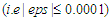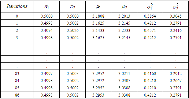
3. Stopping criteria: If stopping rule are satisfied (convergence of parameters and log-likelihood) then we stop, else we set and go back to step 1 and input the updated parameter values for the next iteration. . Where is the number at which convergence or optimality conditions was achieved. Stopping Rule: When all the epsilon values are less than or equal to 0.0001 , or the values of all appears not to be changing significantly from one iterative step to another, then we assume that the EM solution is optimal at that point and cannot be improved upon further. The values of the complete iterations are contained in Table 3 and Table 4 of this paper.

3.5. Result of the Classification Using Data Set 1

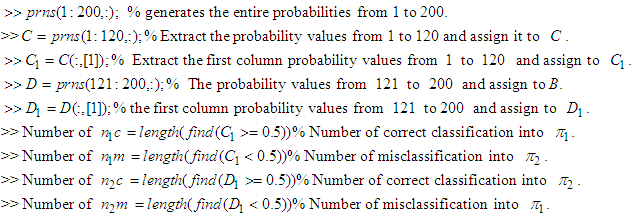
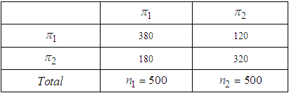
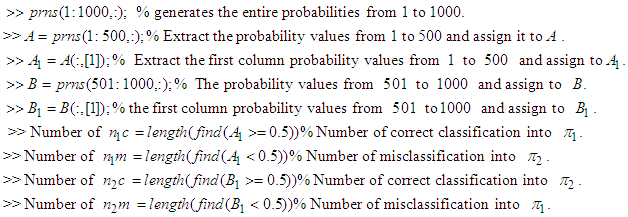
After implementing the classification procedures on the maximized generated posterior probabilities using equation (11) & (12), we obtained the following confusion matrix. See Appendix G for the MATLAB’s source codes for deriving the discriminant values of Table 4 and Table 5.

Table 4

From the obtained confusion matrix in Table 4, we can now compute the apparent error rate to determine the probability of misclassification considering the weights of students. Using equation (12). The apparent error rate is computed as follows:

3.6. Result of the Classification Using Data Set 2

Table 5

Likewise from Table 5, we compute the APER to determine the probability of misclassification considering the babies weights at birth.

4. Conclusions

From this paper, we explained the intricacies of how to estimate the parameters of two combined Gaussian models as well as their classifications using EM Algorithm procedure. We also explained exhaustively the actual estimation of these model parameters using sets of sample data, namely data set for the weights of students and data set 2 for the weights of babies at birth.

Table 2 of our analysis displayed the estimated maximized values of the relevant parameters for the Gaussian mixture model using data set 1, while Table 3 showed the estimated maximized values of the parameters for the mixture model using data set 2. Having a look at the both ends of Table 2 & Table 3, revealed that convergences have been achieved, since the parameter estimates stopped changing significantly at those points and . 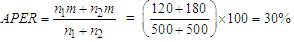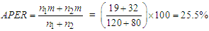Table 4 presents the result of classification using data set 1, whose interpretation implies that we misclassified data set 1 by about 30% failure rate, attributing 70% to correct classification rate. Table 5 at the other hand showed that we misclassified the data set 2 by about 25.5%, having a classification success rate of 74.5%. However, the overall classification efficiency of the Algorithm based on the output of sample data can be considered high, since 70% of Data set 1 and 74.5% of Data set 2 were correctly classified by the Algorithm. These validations achieved by the sample data procedures suggest that EM Algorithm may be useful as early warning statistical tool for parameter estimation and for predicting and classifying the mixture of Gaussians.

Appendix D

The E-step: See William (2008) for Appendix D, E and F.

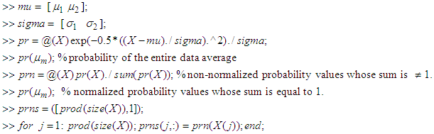
% outputs the normalized posterior probabilities from 1 to 10. Hence, in our Algorithm, we replaced 10 with 1000 or 200 as the case may require. Note: is the entire data for student weights or baby weights at birth. is the entire mean of either data set 1 or data set 2 as the case may also demand.

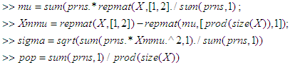
Appendix E

The M-step source codes

Appendix F

MATLAB’s Source codes for the Log-likelihood and the mixing proportions.

Appendix G

MATLAB’s Source codes for the classification/Discriminant Analysis:

For Data Set 1

For Data Set 2